3 Theory

3.1 Summary of this chapter

This chapter discusses causal theory in general and necessity theory in particular. A causal theory helps us understand phenomena, predict effects, and explain empirical findings. The chapter begins (Section 3.2) by discussing the four fundamental elements of a theory: (1) focal unit (e.g., person, organization, country), (2) concepts (varying characteristics of the focal unit), (3) propositions (causal relationships between the concepts), and (4) theoretical domain (generalization to where the theory holds). This is followed by a discussion of parsimonious necessity theories (Section 3.3) and types of necessity theories (Section 3.4), for example a pure necessity theory where all relationships between the concepts are described in terms of necessity, and an embedded necessity theory, where part of the theory has one or more necessity relationships. Next, the direction of a necessity proposition is discussed (Section 3.5), which depends on whether \(X\) and \(Y\) are present/have high value or are absent/have low value. The most common direction is that the presence or high value of \(X\) is necessary for the presence or high value of \(Y\) (high-high direction), which is the default when the direction is not specified. Other possible directions are high-low, low-high, and low-low. The following section (Section 3.6) discusses the expected data pattern when necessity holds. A consequence of a high-high necessary condition is that the upper-left corner in an \(XY\)-plot is expected to be empty. The next section (Section 3.7) discusses the possibility of having double necessity when multiple corners are expected to be empty. The chapter finishes with a discussion of the theoretical meaning of ‘necessary but not sufficient’ (Section 3.8).

3.2 Main elements of a theory

Because there are multiple ways to conceptualize theory, there is no consensus on what a theory is. This book adopts the ‘four elements’ approach to theory (Dul & Hak, 2008), which enables straightforward empirical testing. It uses a broad and inclusive definition of what constitutes a theory, ranging from established theories that are broadly accepted to theoretical assertions by an analyst made in a specific study. Not only academic theories but also ‘theories-in-use’ qualify as a theory. At a minimum, a theory must have four fundamental elements: focal unit, concepts, propositions, and theoretical domain. The focal unit is the object to which the theory applies: country, person, firm, project, etc. The concepts are the variant characteristics of the focal unit representing properties of a phenomenon that can increase or decrease. In NCA, a concept that is the cause is called the ‘condition’ and a concept that is the effect is called the ‘outcome’. The proposition describes the relationship between cause and effect, including the causal explanation. In NCA, the causal relationship is a necessity relationship: \(X\) is necessary for \(Y\), meaning that \(X\) is (almost always) necessary for \(Y\) (Dul, 2024a). The words ‘almost always’ may be omitted from the necessity proposition, allowing both a deterministic and a typicality perspective. As theories in the social sciences are usually semantic (expressed in words), specific levels of the condition (cause) and the outcome (effect) are not specified. The theoretical domain is the set of cases of the focal unit where the theory is supposed to hold, and is defined by the boundary conditions of the theory. A case is one particular example of the focal unit: a specific country, a specific person, etc. For example, a theory that proposes a relationship between physical exercise and stress might be applicable to working adults, but not to children. In that case, the theoretical domain includes only working adults.

For example, the established Theory of Planned Behavior (TPB) explains how an individual’s intention for a specific non-habitual behavior relates to the performance of that behavior (Ajzen, 1991). The focal unit is ‘individual’ or ‘person’, two of its concepts are ‘Intention for the behavior’ (the cause) and ‘Performing the behavior’ (the effect), the proposition describes the causal relationship between these concepts, and one possible theoretical domain is ‘all people in the world’.

The relationship between the two TPB concepts is usually specified as a probabilistic sufficiency relationship, for example ‘Intention to perform a behavior likely to result in Performing the behavior’, or, as the founder of TPB puts it: “As a general rule, the stronger the intention to engage in a behavior, the more likely should be its performance” (Ajzen, 1991, p. 181). Recent interpretations of TPB suggest formulating the relationship between the two concepts in terms of necessity (e.g., Eccarius & Chen, 2024; Frommeyer et al., 2022; Rozenkowska, 2023): for example ‘Intention to perform a behavior is necessary for Performing the behavior’. The key difference between a conventional (probabilistic sufficiency) theory and a necessity theory is the difference in specification of the causal relationship, in other words the causal perspective (Dul, 2024a) that is used to describe the relationship between the concepts (i.e., the proposition).

A theory is only complete if it is accompanied by a plausible substantive explanation of why the cause affects the outcome. For a necessity proposition, the theory should explain (1) why all cases from the theoretical domain with the outcome have the condition, (2) why without the condition, the outcome does not exist, (3) why the absence of the condition is not compensable by other factors (no possibility of substitution), and (4) that the condition precedes the outcome (fulfilling the temporality requirement of causality). Details about how to formulate a formal necessity hypothesis embedded in a necessity theory are explained in Chapter 7. When applying NCA, a necessity theory that causally explains the necessity relationship is essential.

3.3 Parsimonious necessity theories

Necessity theories are inherently parsimonious: single concepts make a strong, actionable prediction: the absence of a necessary condition perfectly predicts the absence of the outcome. Starting with William of Ockham’s parsimony principle²⁰ (also known as Occam’s Razor), many famous scholars including Newton²¹, Einstein²², Popper²³, and Simon²⁴ emphasized the importance of keeping theories simple, such that they are understandable, practically useful, and falsifiable.

Because necessary conditions operate in isolation from the rest of the causal structure (see Section 4.6), even the simplest necessity theory with only one or a few necessary conditions can be actionable. Figure 3.1 shows a necessity theory with two concepts: one condition \(X\) and one outcome \(Y\). To emphasize the necessity perspective used to describe the relationship, nc (necessary cause or necessary condition) is placed above the arrow.

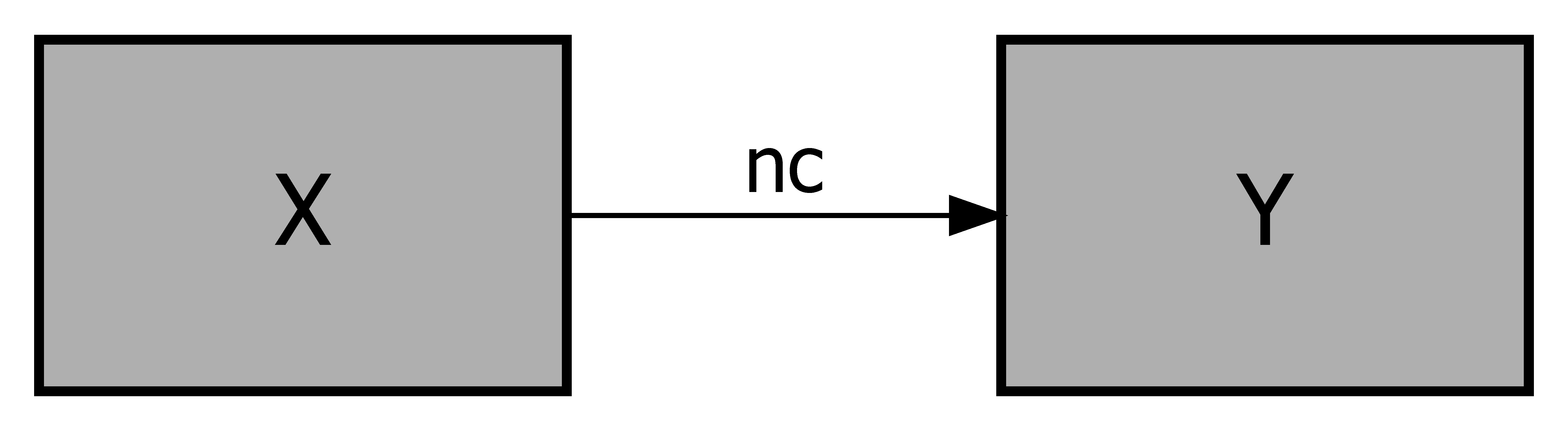
Figure 3.1: Conceptual model of a necessity theory with one condition and one outcome.

It is also possible that multiple concepts (e.g., \(X_1\), \(X_2\), \(X_3\)) are necessary for the same outcome (\(Y\)) as shown in Figure 3.2-left, or that one or more conditions are necessary for several outcomes (e.g., \(Y_1\), \(Y_2\), \(Y_3\)), which is shown in Figure 3.2-right. Note that conditions \(X_1\), \(X_2\), and \(X_3\) are all individual necessary conditions. If any one condition is missing (below its required level) the outcome cannot occur (at its target level), while the presence of all conditions is normally not sufficient for the outcome because other contributing factors must be in place as well.

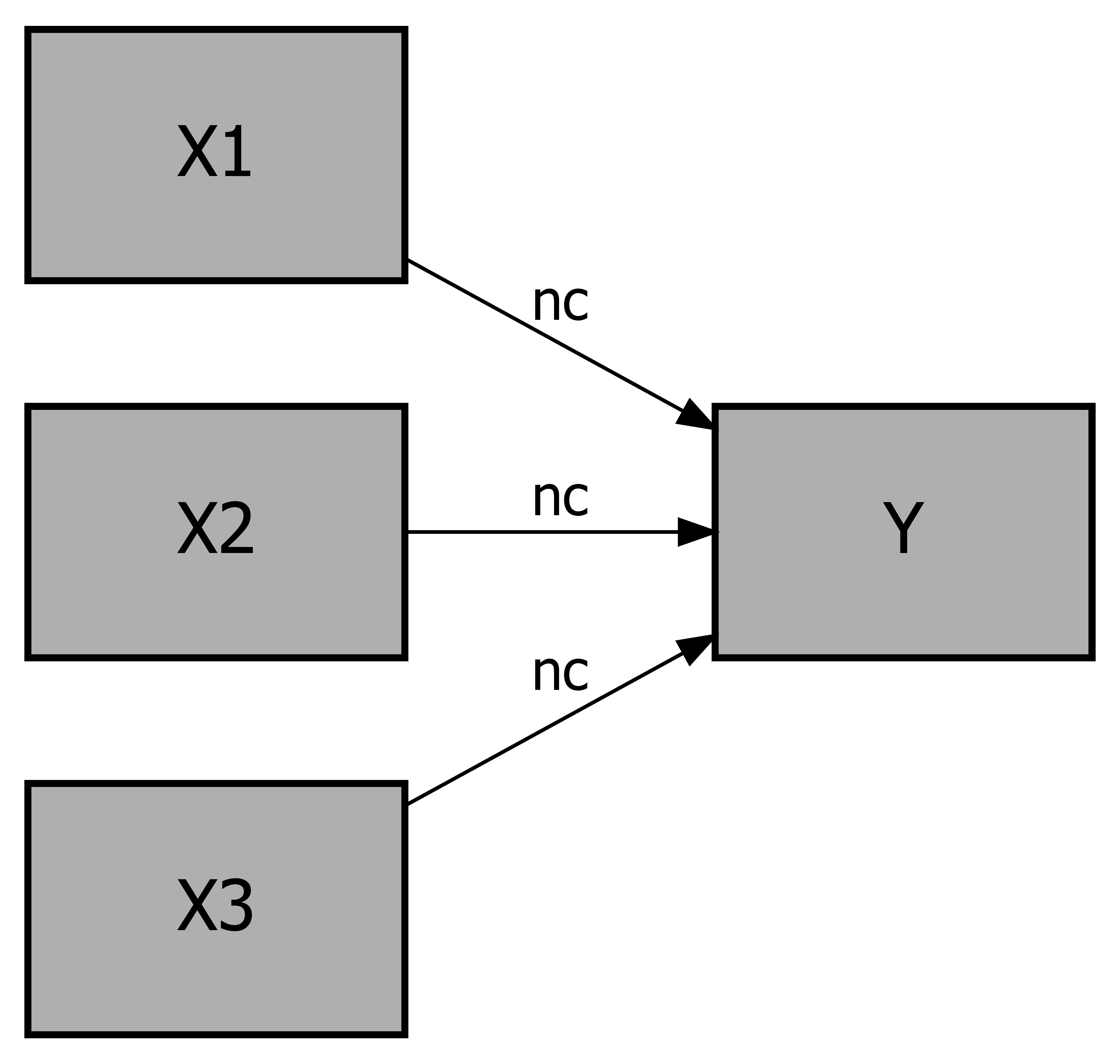
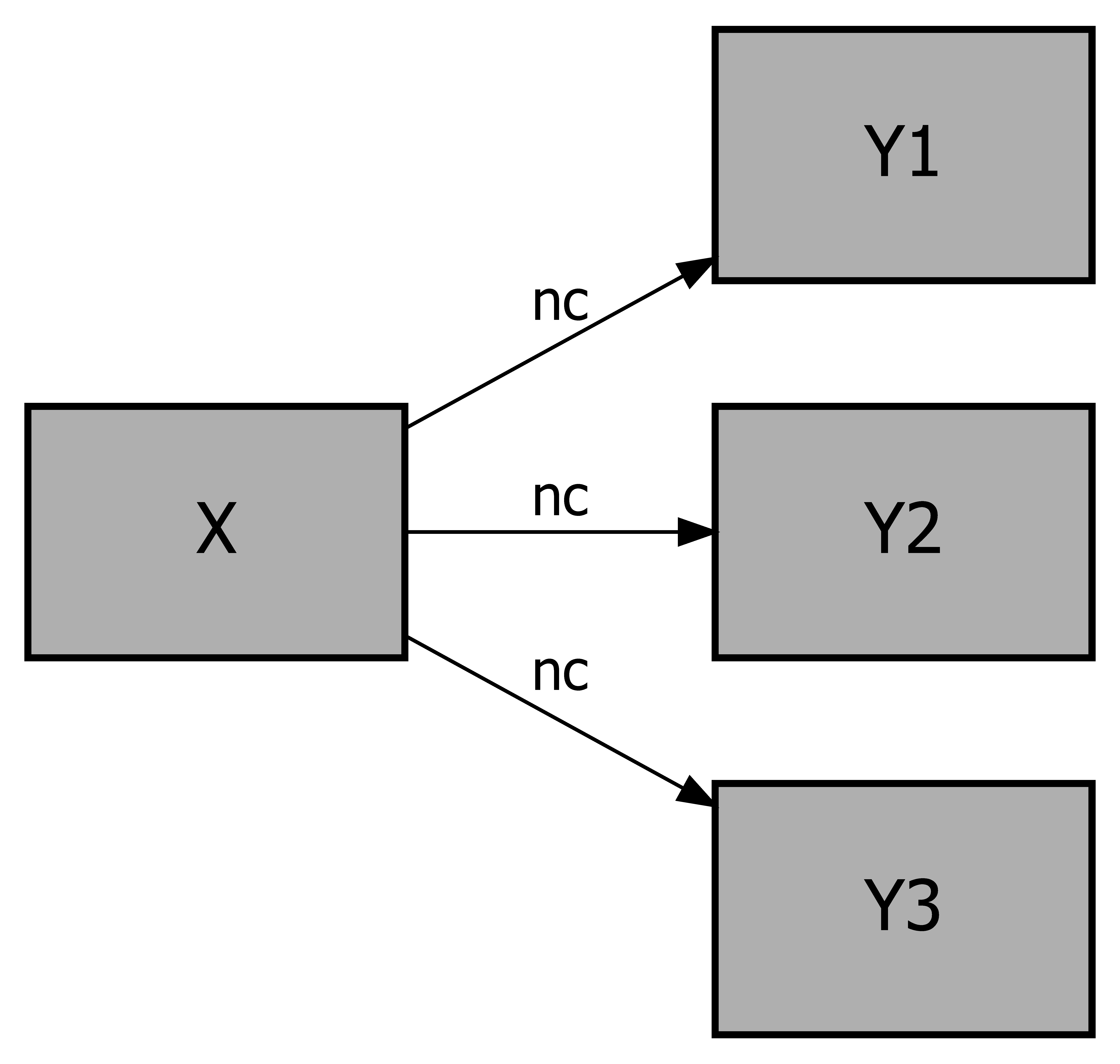
Figure 3.2: Conceptual models of a necessity theory with three conditions and one outcome (Left), and of a theory with one condition and three outcomes (Right).

Furthermore, several necessary conditions can combine into a necessity causal chain where \(X_1\) is necessary for \(X_2\), and \(X_2\) is necessary for \(Y\). This situation is shown in Figure 3.3 and is called ‘chain necessity’ of \(X_1\) for \(Y\). Chain necessity differs from ‘direct necessity’ as shown in Figure 3.1. In the dichotomous necessity-in-kind (NiK) situation, the necessity of \(X_1\) for \(X_2\) and of \(X_2\) for \(Y\) implies the necessity of \(X_1\) for \(Y\). However, in the necessity-in-degree (NiD) situation it is possible that the chain necessity of \(X_1\) for \(Y\) is absent despite the necessity between the elements of the chain (\(X_1\) for \(X_2\) and \(X_2\) for \(Y\)), as discussed in Section 4.6.4.

Figure 3.3: Conceptual model of a chain of necessary conditions. \(X_1\) is necessary for \(X_2\) and \(X_2\) is necessary for \(Y\).

Necessity models are inherently parsimonious. A single necessary condition can stop the outcome, independently of other conditions and other contributing factors. However, in sufficiency-based perspectives, a single factor is seldom enough to produce the outcome. For a probabilistic or configurational sufficiency model, a series of factors are included to model causal complexity. This applies to both probabilistic sufficiency (e.g., structural causal models) and configurational sufficiency (e.g., as in QCA). Parts of the relationships of sufficiency models could (also) be necessity relationships. For the necessity analysis these parts can be isolated (as in Figure 3.1) from the rest of the causal structure and independently be analyzed for necessity (Chapter 11).

3.4 Types of necessity theories

Necessity theories can be classified according to the extent to which necessity propositions are part of the theory. Bokrantz & Dul (2023) distinguish between pure necessity theories, which are theories that consist only of necessity relationships between the concepts and embedded necessity theories, which are theories that consist of a mix of necessity relationships and other relationships (e.g., probabilistic sufficiency or configurational sufficiency). In embedded necessity theories, some of the relationships may be necessity relationships (e.g., \(X_1 \xrightarrow{nc\ } Y\)), whereas others may be probabilistically sufficient relationships (\(X_2 \xrightarrow{+\ } Y\)). It is also possible that one condition has both causal roles in a model such that the presence of \(X\) is necessary for the presence of \(Y\), but also that \(X\) likely increases \(Y\) (\(X \xrightarrow{nc\ ,\ +} Y\)).²⁵

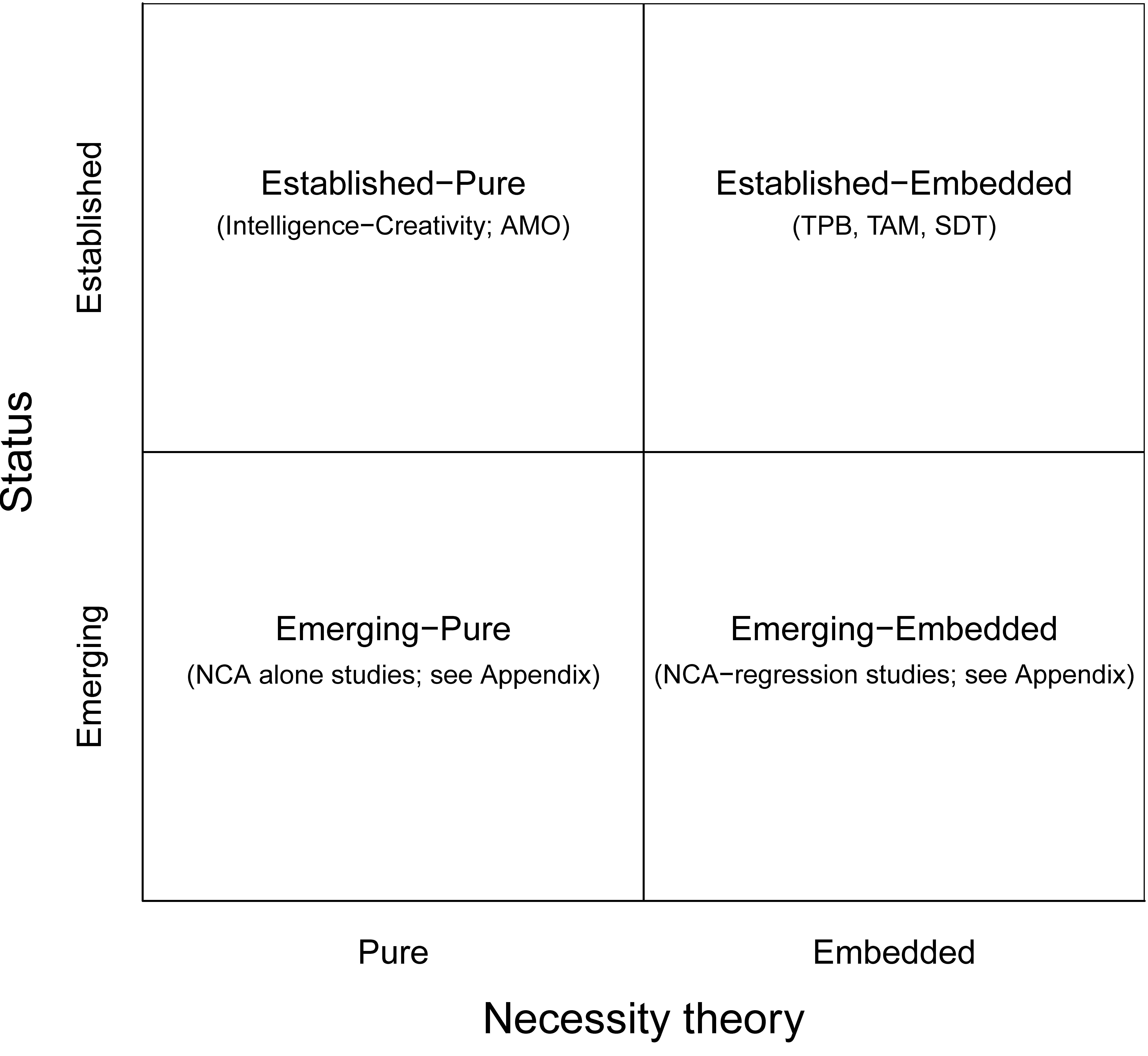
Figure 3.4: Typology of necessity theories with examples. AMO = Ability-Motivation-Opportunity. TPB = Theory of Planned Behavior. TAM = Technology Acceptance Model. SDT = Self-Determination Theory.

Figure 3.4 shows the four possible types of necessity theories by also considering if the necessity theory is established or emerging.
Established pure necessity theories, where all relationships in the theory are necessity relationships as in Figures 3.1, 3.2, and 3.3 in Section 3.2 are relatively scarce. One example is the early theory of Guilford (1967) that intelligence is necessary for creativity. Shortly after NCA was introduced (Dul, 2016b), this theory was empirically tested with NCA and supported (Karwowski et al., 2016). Another established pure necessity theory is the original Ability, Motivation, Opportunity model (AMO) or Motivation, Opportunity, Ability (MOA) model of human behavior. Necessity lies at the core of this theory assuming that A, M, and O are single necessary conditions for behavior.²⁶

Established embedded necessity theories are broadly accepted theories consisting of both necessity and probabilistic sufficiency relationships. Often, these theories are originally formulated as probabilistic sufficiency theories for all their relationships, and revisited to suggest a necessity perspective for one or more relationships. An example is Frommeyer et al. (2022)’s interpretation of one relationship of the Theory of Planned Behavior (TPB): Intention of the behavior is necessary for Performance of the behavior, while keeping the other relationships as probabilistic sufficiency.²⁷ Another example is the Technology Acceptance Model (TAM) that is usually interpreted and studied as a probabilistic sufficiency theory and that was recently revisited with a necessity causal perspective for all relationships while maintaining also the probabilistic sufficiency perspective (e.g., Erdmann & Toro-Dupouy, 2025; Hassan et al., 2025; Kopplin, 2023b; Low & Ramayah, 2023; Richter, Schubring, et al., 2020; D. N. Su et al., 2023).²⁸ Also the Self-Determination Theory (SDT) was recently revisited from the perspective of necessity only (H. Ding & Kuvaas, 2023, 2025) or in combination with the probabilistic sufficiency perspective (Cassia & Magno, 2024). SDT suggests that humans have three basic psychological needs (motivation, competence, relatedness) that must be satisfied for optimal human development and well-being.

Many established theories exist (not shown in Figure 3.4) that could be revisited from a necessity perspective to develop pure or embedded necessity theories because their founders clearly employed necessity causal reasoning to formulate these theories. Examples include Porter’s theory on competitive advantage of nations (Porter, 1985), Wernerfelt’s resource-based view of the firm (Wernerfelt, 1984), Teece’s theory on dynamic capabilities (Teece et al., 1997; Teece, 2007), Rogers’ theory on person-centered psychotherapy (Rogers, 1957), Turner’s framework for project management success (Turner, 2009), and Meehl’s concept of ‘specific etiology’ in medicine (Meehl, 1962). Until recently, such theories were mostly tested using regression-based methods that implicitly assume probabilistic sufficiency, suggesting theory-method misfit (Table 11.1). With NCA available, testing necessity with a dedicated methodology becomes possible.

Since the introduction of NCA, the number of emerging pure necessity theories has risen. Appendix C.1 includes examples of NCA studies in which only necessity relationships are theoretically formulated and tested with NCA. After replication and further theorizing, these emerging necessity theories may become established necessity theories. An example of an empirical study with an emerging pure necessity theory is a study by B. Yan et al. (2023) that proposes and finds four necessary conditions for a country’s high level of early COVID-19 mortality rate: high levels of a delayed first response, political decentralization, elderly populations, and urbanization. An example of a theoretical study with an emerging pure necessity theory is the study by Andrevski & Miller (2022) about defining the concept ‘strategic forbearance’. When firms are attacked by competitors, forbearance is defined by three necessary conditions: the presence of awareness of the attack, the presence of capabilities to react, and the absence of a motivation to react.

Many studies formulate emerging embedded necessity theories. Such studies often start with a probabilistic sufficiency theory based on earlier empirical regression-based studies and then suggest that one or more of the relationships could (also) be formulated as necessity relationships. In an empirical study W. Lee & Jeong (2021) propose an emerging embedded necessity theory in which two dimensions of tourist happiness experience (Hedonic enjoyment and Personal expressiveness) are related to Satisfaction (customer’s judgment about their fulfillment with a product or service) and Place attachment (bonding between individuals and places). This is shown in the conceptual model of Figure 3.5. By conducting both NCA and structural equation modeling (SEM), they conclude that Hedonic enjoyment (pleasure, comfort) has both a necessity relationship and a probabilistic sufficiency relationship with Satisfaction, but only a necessity relationship with Place attachment. Furthermore, they conclude that Personal expressiveness (a subjective experience of self-realization that one is acting in such a way that one is truly being oneself) has no probabilistic sufficiency relationship with Satisfaction, and both a necessity relationship and a probabilistic sufficiency relationship with Place attachment. Other examples of emerging embedded necessity theories may be found in empirical studies that apply NCA in combination with regression-based methods (Tables C.2, C.3, and C.4 in Appendix C). Liehr & Hauff (2022) propose in a theoretical study an emerging embedded necessity theory about leadership competencies for employee innovative behavior. They review a large number of competencies that contribute to innovative behavior and conclude that three competencies (according to the literature) have a probabilistic sufficiency relationship with innovative behavior but are not necessary (rewards, sharing expertise, resource management) and four competencies are (also) necessary: providing support, communicating a vision, granting autonomy and discretion, and providing feedback.

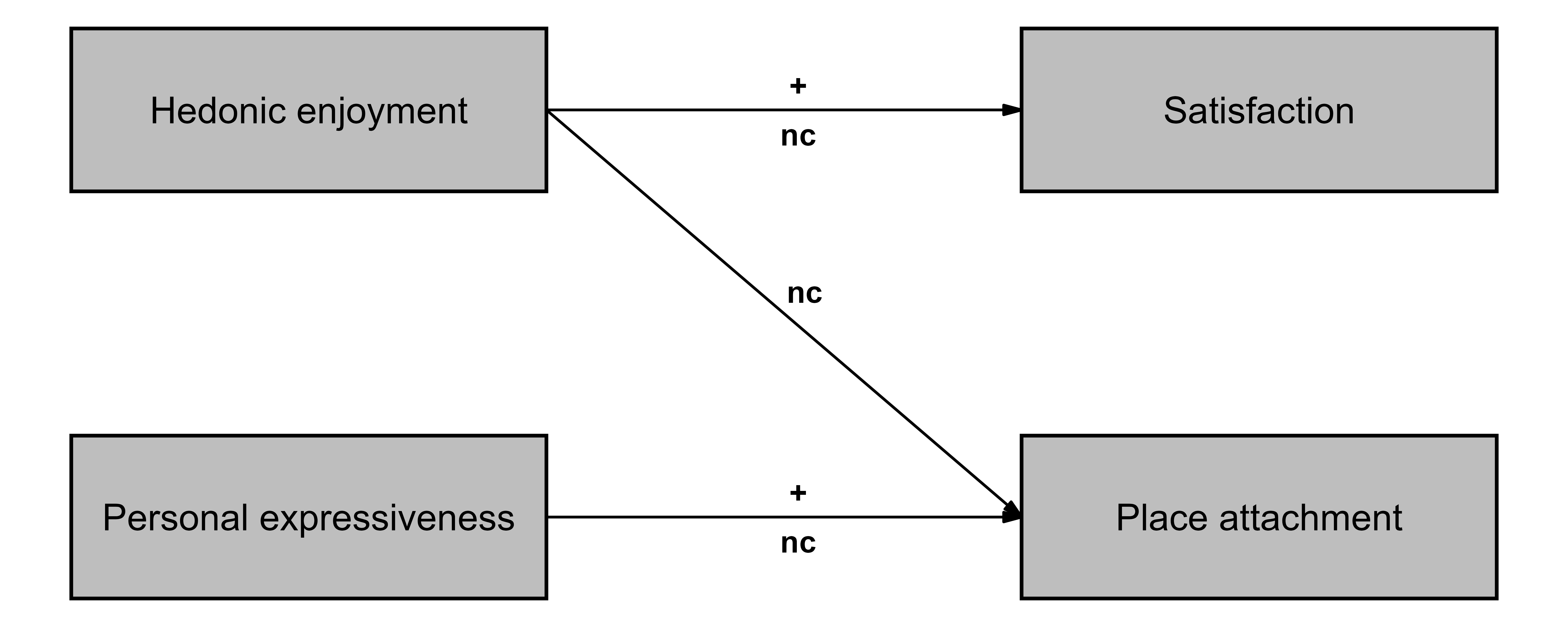
Figure 3.5: Example of an emerging embedded necessity theory for the effect of two dimensions of happiness experiences (Hedonic enjoyment and Personal expressiveness) on two outcomes (Satisfaction and Place attachment). The symbol + represents a positive probabilistic relationship and the symbol nc represents a necessity relationship with high-high direction (After W. Lee & Jeong, 2021).

3.5 Direction of a necessity relationship

In Figure 3.5 the direction of the probabilistic sufficiency relationship is given by a + symbol above the arrow. This convention indicates a positive effect: \(X\) increases \(Y\) or \(X\) has a positive effect on \(Y\) or more precisely, that a higher value of \(X\) increases the probability of a higher value of \(Y\). Similarly, a − symbol indicates a negative effect: \(X\) decreases or has a negative effect on \(Y\); a higher value of \(X\) decreases the probability of a higher value of \(Y\).

Such single symbols do not convey meaning for a necessity relationship. In a necessity proposition the direction is not described by a verb as in \(X\) increases \(Y\) or \(X\) has a positive effect on \(Y\). For a necessity proposition a noun or adverb (or a combination) is used to describe relationships between levels of \(X\) and \(Y\). For example, in the dichotomous situation absence of \(X\) is necessary for presence of \(Y\) or in the continuous situation low level of \(X\) is necessary for high level of \(Y\). For a necessity relationship four possible directions exist (Figure 3.6).

First, for a necessary condition with a high-high direction, the presence/high value of \(X\) is necessary for presence/high value of \(Y\). This is symbolized as (Figure 3.6). For example, high level of Urbanization is necessary for a high level of Early COVID-19 mortality (B. Yan et al., 2023).

Second, for a necessary condition with a low-high direction, the absence/low value of \(X\) is necessary for the presence/high value of \(Y\) (). For example, low Intensity of production is necessary for high Environmental sustainability in agriculture (Lankoski & Lankoski, 2023).

Third, for a necessary condition with a high-low direction, the presence/high value of \(X\) is necessary for the absence/low value of \(Y\) (). For example, the presence/high value of social support is necessary for the absence/low value of stress.

Fourth, for a necessary condition with a low-low direction, the absence/low value of \(X\) is necessary for the absence/low value of \(Y\) (). For example, the absence of rain is necessary for the absence of a wet surface.

The third and fourth formulations of a necessary condition are less common than the first and second. Often the absence/low value of the outcome is redefined as the presence/high level of the opposite of the outcome. For example, the presence/high value of social support is necessary for the presence/high value of relaxation or the absence of rain is necessary for the presence of a dry surface. Thus, the direction of the necessity relationship depends on the definition of the concepts that are part of the proposition.

In the absence of a specified direction, the implied direction is , as shown in Figure 3.5. Throughout this book, the default assumption is the direction, unless stated otherwise.

Figure 3.6 shows the four possible conceptual models depending on the direction of the necessity relationship.

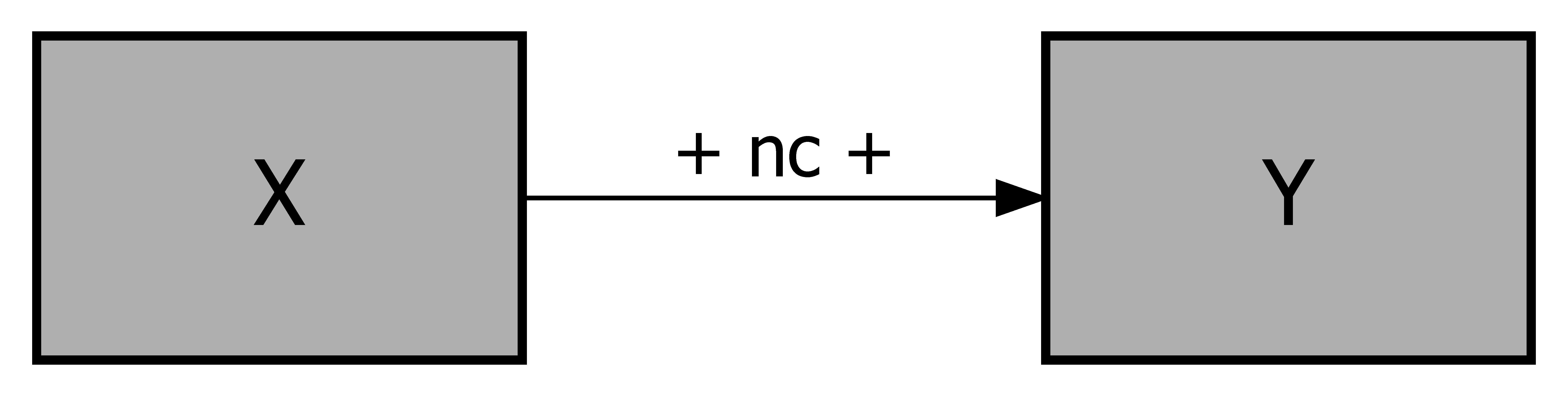
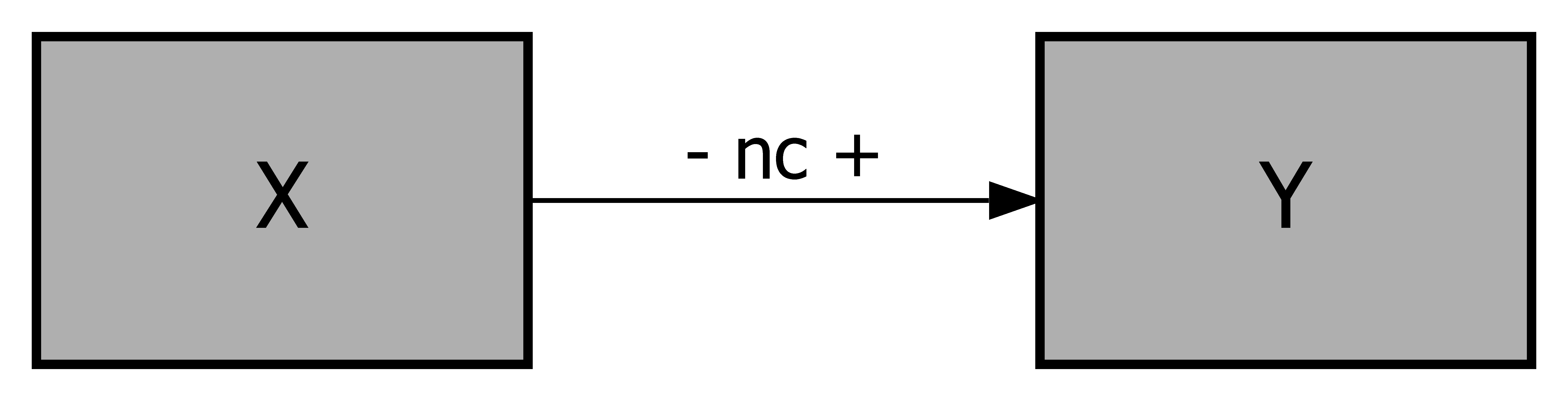
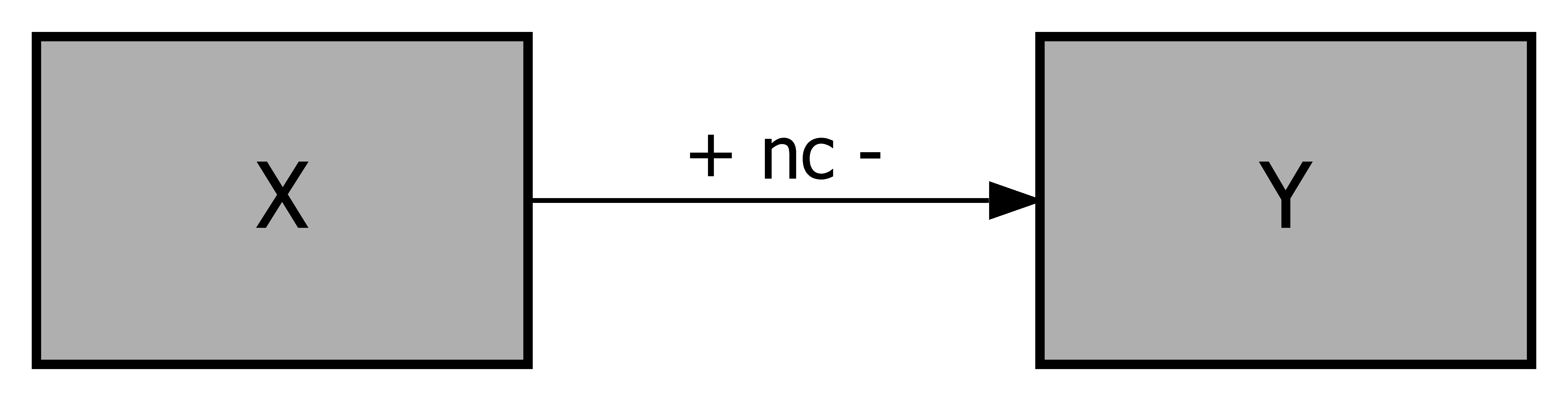
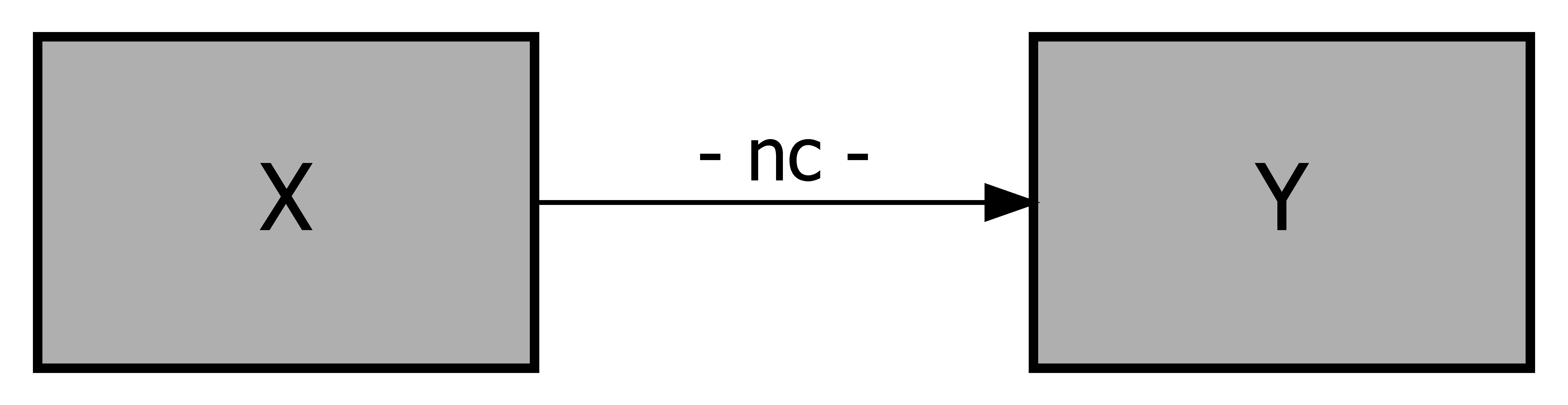
Figure 3.6: Conceptual models for necessary conditions. Top-Left: high-high = presence/high value of \(X\) is necessary for presence/high value of \(Y\). Top-Right: low-high = absence/low value of \(X\) is necessary for presence/high value of \(Y\). Bottom-Left: high-low = presence/high value of \(X\) is necessary for absence/low value of \(Y\). Bottom-Right: low-low = absence/low value of \(X\) is necessary for absence/low value of \(Y\).

Figure 3.7: \(XY\)-tables showing empty corners without observations depending on the direction of the necessity relationship. Top-Left: high-high = presence of \(X\) is necessary for presence of \(Y\). Top-Right: low-high = absence of \(X\) is necessary for presence of \(Y\). Bottom-Left: high-low = presence of \(X\) is necessary for absence of \(Y\). Bottom-Right: low-low = absence of \(X\) is necessary for absence of \(Y\).

3.6 Expected empty corner

Depending on the direction of necessity, different corners in the \(XY\)-table or \(XY\)-plot are expected to be empty. For the dichotomous situation, the \(XY\)-table of Figure 2.1-right illustrates necessity causality when the presence of \(X\) is necessary for the presence of \(Y\). Corner 1 cannot have observations (points, cases) whereas the other corners may have observations. This is also shown in Figure 3.7-top-left. In Figure 3.7 rows represent the two values of the outcome \(Y\) (Absent/Present), and columns the two values of the condition \(X\). The condition \(X\) increases to the right, and the outcome \(Y\) increases upward. Each corner in the table represents a certain combination of \(X\) and \(Y\). For example, the upper-left corner represents absence of \(X\) and presence of \(Y\). A gray corner with a black dot indicates that the corner may contain observations. A white corner without dots indicates that no observations are possible.

When the presence of \(X\) is necessary for the presence of \(Y\), the upper-left corner is empty. This corresponds to the necessity statement ‘if not \(X\), then not \(Y\)’ (see the necessity statement of expression (2.6) in Chapter 2). The outcome is absent when the condition is absent. This means that the upper-left corner does not have observations, and that the lower-left corner has observations. Similarly, when the outcome is present, the condition must also be present: the upper-right corner has observations. The content of the lower-right corner is irrelevant for necessity: this corner may or may not have observations when the necessary condition applies. For necessity, the emptiness of the upper-left corner is essential.

For other directions of the necessity relationship, other corners in the \(XY\)-table remain empty when necessity applies. When necessity applies, the upper-right corner remains empty. Similarly, for necessity, the lower-left corner is empty, and for necessity, the lower-right corner stays unoccupied. Therefore, the empty corner depends on how the necessary condition is formulated in the theory (and how the direction of the axes and the concepts are defined). Each formulation of the necessity proposition results in a specific corner of the \(XY\)-table being empty, referred to as the expected empty corner.

For the continuous situation, Figure 3.8 shows the four directions and corresponding empty corners. Here an \(XY\)-plot instead of an \(XY\)-table is used as a visualization method for representing that a low/high value of the condition is necessary for a low/high value of the outcome. The condition \(X\) increases to the right, and the outcome \(Y\) increases upward. Each corner in the plot represents a certain combination of low/high \(X\)- and \(Y\)-values. For example, the upper-left corner represents low level of \(X\) and high level of \(Y\). A gray area indicates that the area may contain observations.

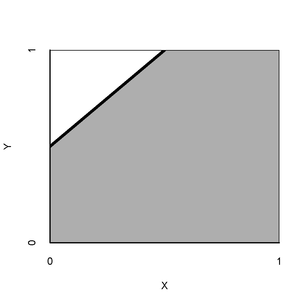
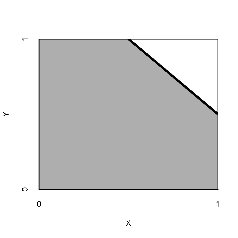
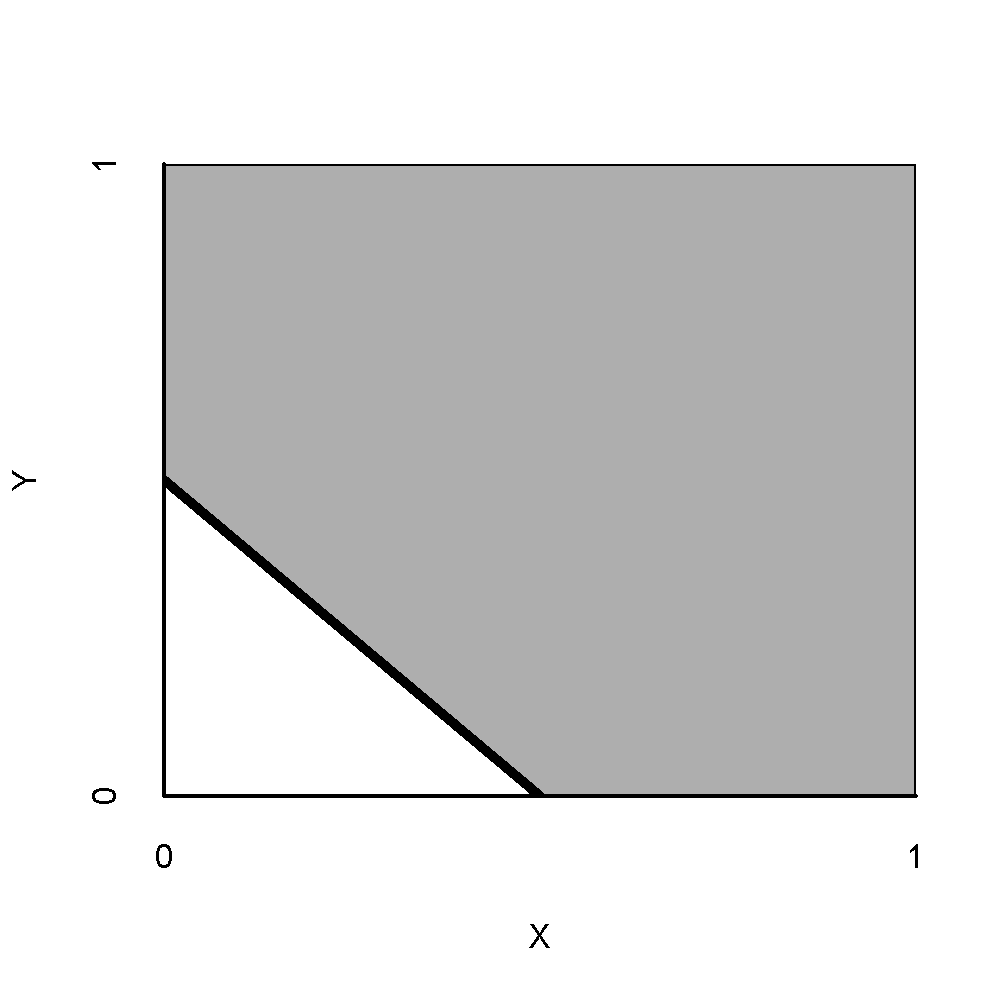
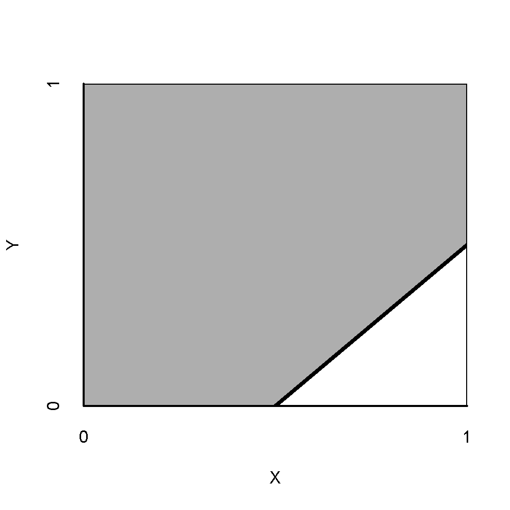
Figure 3.8: \(XY\)-plots showing the direction of a necessity relationship. Top-Left: a high value of \(X\) is necessary for a high value of \(Y\) (+ nc +, high-high). Top-Right: a low value of \(X\) is necessary for a high value of \(Y\) (- nc +, low-high). Bottom-Left: a high value of \(X\) is necessary for a low value of \(Y\) (+ nc -, high-low). Bottom-Right: a low value of \(X\) is necessary for a low value of \(Y\) (- nc -, low-low).

3.7 Double necessity

It is possible that a single factor has two necessity relationships with the outcome at the same time, implying that more than one corner is expected to be empty. When the concepts are continuous, it is possible that two adjacent corners are empty. This allows theorizing that an optimum (not low, not high) level of \(X\) is necessary for a high level of \(Y\), implying that the upper-left and the upper-right corners are expected to be empty (Figure 3.9-left). For example, in team performance, moderate levels of conflict (\(X\)) may be necessary for high team innovation performance (\(Y\)). Low conflict leads to groupthink, which may limit performance; high conflict leads to dysfunction, which also limits team innovation performance. Therefore, a moderate level of conflict enables teams to challenge each other productively, providing the possibility for high innovation performance.
Similarly, it may be theorized that an optimum (not low, not high) level of \(X\) is necessary for a low level of \(Y\), implying that the lower-left and lower-right corners are expected to be empty (Figure 3.9-right). For example, in stress management, moderate levels of workload (\(X\)) may be necessary for low employee burnout (\(Y\)). Low workload can result in boredom and lack of purpose, which may limit the possibility of low burnout; high workload can cause stress and exhaustion, which also limits the possibility of low burnout. Therefore, a moderate workload is necessary for low burnout because both too low and too high workload create psychological strain that prevents burnout from remaining low.

Figure 3.9: \(XY\)-plot showing an optimum level of the necessary condition. Left: An optimum level of \(x_{c1} <x < x_{c2}\) is necessary for a high level of \(y = y_c\). Right: An optimum level of \(x_{c1} < x < x_{c2}\) is necessary for a low level of \(y = y_c\).

It is also possible to theorize that a high level of \(X\) is necessary for an extreme (low or high) level of \(Y\). Then the upper-left and the lower-left corners are expected to be empty (Figure 3.10-left). Similarly, it may be theorized that a low level of \(X\) is necessary for an extreme (low or high) level of \(Y\). Then the upper-right and the lower-right corners are expected to be empty (Figure 3.10-right).

Figure 3.10: \(XY\)-plot showing necessity for an extreme level of the outcome. Left: A high level of \(x > x_c\) is necessary for an extreme (low or high) level of \(y = y_{c1}\) or \(y = y_{c2}\). Right: A low level of \(x < x_c\) is necessary for an extreme (low or high) level of \(y = y_{c1}\) or \(y = y_{c2}\).

The situations shown in Figures 3.9 and 3.10 do not have dichotomous equivalents, as this would imply that the outcome or the condition is always absent (Figure 3.11-top-left) or always present (Figure 3.11-top-right), or that the condition is always present (Figure 3.11-bottom-left), or always absent (Figure 3.11-bottom-right).

Figure 3.11: \(XY\)-tables showing two adjacent empty corners without observations. Top-Left: presence of \(Y\) is not possible. Top-Right: absence of \(Y\) is not possible. Bottom-Left: absence of \(X\) is not possible. Bottom-Right: presence of \(X\) is not possible.

When two opposite corners are empty, as shown in Figure 3.12-left, two claims apply: the presence/high level of \(X\) is necessary for the presence/high level of \(Y\) (empty upper-left corner) and that the absence/low level of \(X\) is necessary for the absence/low level of \(Y\) (empty lower-right corner). Similarly, it may be theorized that the absence/low level of \(X\) is necessary for the presence/high level of \(Y\) (empty upper-right corner) and that the presence/high level of \(X\) is necessary for the absence/low level of \(Y\) (empty lower-left corner). This is shown in Figure 3.12-right. This situation has dichotomous equivalents, as shown in Figure 3.13.

Figure 3.12: Double necessity. Left: A high level of \(x > x_{c1}\) is necessary for a high level of \(y = y_{c1}\), and a low level of \(x < x_{c2}\) is necessary for a low level of \(y = y_{c2}\). Right: A low level of \(x < x_{c1}\) is necessary for a high level of \(y = y_{c1}\), and a high level of \(x > x_{c2}\) is necessary for a low level of \(y = y_{c2}\).

Figure 3.13: \(XY\)-tables showing two opposite empty corners without observations. Left: the presence of \(X\) is necessary for the presence of \(Y\) and the absence of \(X\) is necessary for the absence of \(Y\). Right: the absence of \(X\) is necessary for the presence of \(Y\) and the presence of \(X\) is necessary for the absence of \(Y\).

3.8 The meaning of ‘necessary but not sufficient’

To understand what necessary but not sufficient means, this section first explains what is meant by necessary and sufficient. In the dichotomous situation, ‘necessary and sufficient’ means that the upper-left corner and the lower-right corner of the \(XY\)-plot are both empty. This is shown in Figure 3.13, which is interpreted as a double necessity relationship of \(X\) for \(Y\): a necessity relationship where the presence of \(X\) is necessary for the presence of \(Y\) (upper-left corner empty) and a necessity relationship where the absence of \(X\) is necessary for the absence of \(Y\) (lower-right corner empty). By logic, in the dichotomous situation the second relationship can be reformulated as a sufficiency relationship where the presence of \(X\) is sufficient for the presence of \(Y\), as shown in Figure 2.1-left. The first relationship (necessity) and the second relationship (sufficiency) now have the same \(X\)-value (presence) and the same \(Y\)-value (presence). This allows a single statement that the presence of \(X\) is necessary and sufficient for the presence of \(Y\). If the sufficiency relationship does not hold, the formulation of the combined relationship would be: the presence of \(X\) is necessary but not sufficient for the presence of \(Y\). This means that the lower-right corner is not empty.

In discrete and continuous situations, necessity and sufficiency are more complex. Like in the dichotomous situation, the upper-left corner and the lower-right corner are both empty. This is shown in Figure 3.12-left, which is interpreted as a double necessity relationship of \(X\) for \(Y\): a necessity relationship where a high level of \(X\) is necessary for a high level of \(Y\) (upper-left corner empty) and a necessity relationship where a low level of \(X\) is necessary for a low level of \(Y\) (lower-right corner empty). By logic, the second relationship can again be reformulated as a sufficiency relationship: a not-low level of \(X\) is sufficient for a not-low level of \(Y\). However, a ‘not-low’ level is usually not the same as a ‘high’ level. For example, in Figure 3.12-left, level \(X = x_{c1}\) is necessary for level \(Y = y_{c1}\), whereas level \(X = x_{c2}\) is sufficient for level \(Y = y_{c2}\). There are no common \(X\)-levels and common \(Y\)-levels that would allow a single statement that level \(X = x_{c}\) is necessary and sufficient for level \(Y = y_{c}\), unless the upper ceiling line and the lower ceiling line (floor line) overlap or intersect at the point (1,1). If the lines overlap there are only observations on the ceiling line and the necessity and sufficiency statement holds for all observations. If the lines intersect at point [1,1], only at that point the necessity and sufficiency statement holds. Both situations are, however, exceptional.

In all other situations the statement that level \(X = x_{c}\) is necessary but not sufficient for level \(Y = y_{c}\) has a broader meaning than that the lower-right corner is not empty. If the lower-right corner can have observations, observations are normally possible in the entire area below the ceiling line, not just in the lower-right corner. This allows a single statement that \(X = x_{c}\) is necessary but not sufficient for \(Y = y_{c}\). When \(X = x_{c}\), no observations are above point \(C\) on the ceiling line, whereas observations below point \(C_1\) are possible. In other words, for a given level \(X = x_{c}\), it is not possible to have values of \(Y > y_{c}\) (necessity applies) but it is possible to have values \(Y \leq y_{c}\) (“non-sufficiency” applies). Consequently, where in the dichotomous situation the statement \(X\) is necessary but not sufficient for \(Y\) means that observations are possible in the lower-right corner, in the discrete and continuous situations it means that there are observations below the ceiling line. NCA focuses on the identification of necessity (rather than on the identification of non-sufficiency) in any corner of the \(XY\)-table or the \(XY\)-plot. If the focus is on the lower-right corner, the emptiness of this corner is interpreted as indicating that the absence or a low level of \(X\) is necessary for the absence or a low level of \(Y\).

References

Ajzen, I. (1991). The theory of planned behavior. Organizational Behavior and Human Decision Processes, 50, 179–211. https://doi.org/10.1016/0749-5978(91)90020-T

Andrevski, G., & Miller, D. (2022). Forbearance: Strategic nonresponse to competitive attacks. Academy of Management Review, 47(1), 59–74. https://doi.org/10.5465/amr.2018.0248

Bokrantz, J., & Dul, J. (2023). Building and testing necessity theories in supply chain management. Journal of Supply Chain Management, 59, 48–65. https://doi.org/10.1111/jscm.12287

Cassia, F., & Magno, F. (2024). The value of self-determination theory in marketing studies: Insights from the application of PLS-SEM and NCA to anti-food waste apps. Journal of Business Research, 172, 114454. https://doi.org/10.1016/j.jbusres.2023.114454

Ding, H., & Kuvaas, B. (2023). Using necessary condition analysis in managerial psychology research: Introduction, empirical demonstration and methodological discussion. Journal of Managerial Psychology, 38(4), 260–272. https://doi.org/10.1108/JMP-12-2022-0637

Ding, H., & Kuvaas, B. (2025). Exploring the necessary roles of basic psychological needs at work: A necessary condition analysis. Journal of Occupational and Organizational Psychology, 98(1), e70012. https://doi.org/10.1111/joop.70012

Dul, J. (2016b). Necessary Condition Analysis (NCA): Logic and methodology of “necessary but not sufficient” causality. Organizational Research Methods, 19(1), 10–52. https://doi.org/10.1177/1094428115584005

Dul, J. (2024a). A different causal perspective with Necessary Condition Analysis. Journal of Business Research, 177, 114618. https://doi.org/10.1016/j.jbusres.2024.114618

Dul, J., & Hak, T. (2008). Case Study Methodology in Business Research. Routledge. https://www.routledge.com/Case-Study-Methodology-in-Business-Research/Dul-Hak/p/book/9780750681964

Eccarius, T., & Chen, C.-F. (2024). Examining trust as a critical factor for the adoption of electric vehicle sharing via necessary condition analysis. Technological Forecasting and Social Change, 208, 123681. https://doi.org/10.1016/j.techfore.2024.123681

Einstein, A. (1934). On the method of theoretical physics. Philosophy of Science, 1(2), 163–169. https://doi.org/10.1086/286316

Erdmann, A., & Toro-Dupouy, L. (2025). The influence of the institutional environment on AI adoption in universities: Identifying value drivers and necessary conditions. European Journal of Innovation Management, 28, 4365–4398. https://doi.org/10.1108/ejim-04-2024-0407

Frommeyer, B., Wagner, E., Hossiep, C. R., & Schewe, G. (2022). The utility of intention as a proxy for sustainable buying behavior – a necessary condition analysis. Journal of Business Research, 143, 201–213. https://doi.org/10.1016/j.jbusres.2022.01.041

Guilford, J. P. (1967). The nature of human intelligence. McGraw-Hill. https://www.worldcat.org/title/nature-of-human-intelligence/oclc/204270

Hassan, M. S., Mai, N. H., Wahab, N. S. A., Amin, M. B., Hassan, M. M., & Oláh, J. (2025). Decentralized fintech platforms adoption intention in cyber risk environment among GenZ: A dual-method approach using PLS-SEM and necessary condition analysis. Computers in Human Behavior Reports, 18, 100687. https://doi.org/10.1016/j.chbr.2025.100687

Hauff, S., Guerci, M., Dul, J., & Rhee, H. van. (2021). Exploring necessary conditions in HRM research: Fundamental issues and methodological implications. Human Resource Management Journal, 31(1), 18–36. https://doi.org/10.1111/1748-8583.12231

Karwowski, M., Dul, J., Gralewski, J., Jauk, E., Jankowska, D. M., Gajda, A., Chruszczewski, M. H., & Benedek, M. (2016). Is creativity without intelligence possible? A necessary condition analysis. Intelligence, 57, 105–117. https://doi.org/10.1016/j.intell.2016.04.006

Kopplin, C. S. (2023b). Chatbots in the workplace: A technology acceptance study applying uses and gratifications in coworking spaces. Journal of Organizational Computing and Electronic Commerce, 32, 232–257. https://doi.org/10.1080/10919392.2023.2215666

Lankoski, J., & Lankoski, L. (2023). Environmental sustainability in agriculture: Identification of bottlenecks. Ecological Economics, 204, 107656. https://doi.org/10.1016/j.ecolecon.2022.107656

Lee, W., & Jeong, C. (2021). Distinctive roles of tourist eudaimonic and hedonic experiences on satisfaction and place attachment: Combined use of SEM and necessary condition analysis. Journal of Hospitality and Tourism Management, 47, 58–71. https://doi.org/10.1016/j.jhtm.2021.02.012

Liehr, J., & Hauff, S. (2022). Must have or nice to have? Necessary leadership competencies to enable employees’ innovative behaviour. International Journal of Innovation Management, 26(10), 2250070. https://doi.org/10.1142/S1363919622500700

Low, M. P., & Ramayah, T. (2023). It isn’t enough to be easy and useful! Combined use of SEM and necessary condition analysis for a better understanding of consumers’ acceptance of medical wearable devices. Smart Health, 27, 100370. https://doi.org/10.1016/j.smhl.2022.100370

Meehl, P. E. (1962). Schizotaxia, schizotypy, schizophrenia. American Psychologist, 17(12), 827–838. https://doi.org/10.1037/h0041029

Newton, I. (1687). Philosophiæ naturalis principia mathematica. Royal Society. https://tile.loc.gov/storage-services/service/gdc/gdcwdl/wd/l_/17/84/2/wdl_17842/wdl_17842

Ockham, W. of. (1323). Summa logicae.

Popper, K. (1959). The logic of scientific discovery. Hutchinson.

Porter, M. E. (1985). Competitive advantage of nations: Creating and sustaining superior performance. The Free Press.

Richter, N. F., Schubring, S., Hauff, S., Ringle, C. M., & Sarstedt, M. (2020). When predictors of outcomes are necessary: Guidelines for the combined use of PLS-SEM and NCA. Industrial Management & Data Systems, 120(12), 2243–2267. https://doi.org/10.1108/IMDS-11-2019-0638

Rogers, C. R. (1957). The necessary and sufficient conditions of therapeutic personality change. Journal of Consulting Psychology, 21(2), 95. https://doi.org/10.1037/0033-3204.44.3.240

Rozenkowska, K. (2023). Theory of planned behavior in consumer behavior research: A systematic literature review. International Journal of Consumer Studies, 47(6), 2670–2700. https://doi.org/10.1111/ijcs.12970

Siemsen, E., Roth, A. V., & Balasubramanian, S. (2008). How motivation, opportunity, and ability drive knowledge sharing: The constraining-factor model. Journal of Operations Management, 26(3), 426–445. https://doi.org/10.1016/j.jom.2007.09.001

Simon, H. A. (1957). Models of man: Social and rational. Wiley.

Su, D. N., Nguyen-Phuoc, D. Q., Tran, P. T. K., Van Nguyen, T., Luu, T. T., & Pham, H.-G. (2023). Identifying must-have factors and should-have factors affecting the adoption of electric motorcycles – a combined use of PLS-SEM and NCA approach. Travel Behaviour and Society, 33, 100633. https://doi.org/10.1016/j.tbs.2023.100633

Teece, D. J. (2007). Explicating dynamic capabilities: The nature and microfoundations of (sustainable) enterprise performance. Strategic Management Journal, 28(13), 1319–1350. https://doi.org/10.1002/smj.640

Teece, D. J., Pisano, G., & Shuen, A. (1997). Dynamic capabilities and strategic management. Strategic Management Journal, 18(7), 509–533. https://doi.org/10.1002/(SICI)1097-0266(199708)18:7<509::AID-SMJ882>3.0.CO;2-Z

Turner, J. R. (2009). The Handbook of Project-based Management. The McGraw-Hill Companies, Inc. https://www.accessengineeringlibrary.com/content/book/9780071549745

Tuuli, M. M., & Rhee, H. van. (2021). How ability, motivation, and opportunity drive individual performance behaviors in projects: Tests of competing theories. Journal of Management in Engineering, 37(6), 04021070. https://doi.org/10.1061/(ASCE)ME.1943-5479.0000969

Van Rhee, H., & Dul, J. (2017). The limiting-factor theory: AMO-factors individually necessary and jointly sufficient for behavior. Academy of Management Proceedings, 2017, 16432. https://doi.org/10.5465/AMBPP.2017.16432abstract

Wernerfelt, B. (1984). A resource-based view of the firm. Strategic Management Journal, 5(2), 171–180. https://doi.org/10.1002/smj.4250050207

Yan, B., Liu, Y., Chen, B., Zhang, X., & Wu, L. (2023). What matters the most in curbing early COVID-19 mortality? A cross-country Necessary Condition Analysis. Public Administration, 101(1), 71–89. https://doi.org/10.1111/padm.12873

---

20. An important element of parsimony is that theories should be simple: “… frustra fit per plura, quod potest fieri per pauciora” (it is pointless to do with more what can be done with fewer) (Ockham, 1323).↩︎

21. “Causas rerum naturalium non plures admitti debere, quam quae & verae sint & earum phaenomenis explicandis sufficiant” (the causes of natural things should not be multiplied beyond what is true and sufficient to explain their appearances) (Newton, 1687).↩︎

22. “It can scarcely be denied that the supreme goal of all theory is to make the irreducible basic elements as simple and as few as possible without having to surrender the adequate representation of a single datum of experience” (Einstein, 1934).↩︎

23. “We do not seek highly probable theories, but explanations; and the best explanations are often simple explanations” (K. Popper, 1959).↩︎

24. “Simplicity is not an optional accessory in human thought and action; it is a necessity” (Simon, 1957).↩︎

25. See also Section 3.5 for various possible directions of necessity and probabilistic sufficiency relationships and their notation. It is possible that \(X\) is necessary for \(Y\) with or without being also probabilistically sufficient for \(Y\). NCA only considers the necessity role of the concept. Assuming a double role of a concept is commonplace in theories that are analyzed both by NCA and a regression-based model (see Section 11.3).↩︎

26. In this framework it is also assumed that the three necessary conditions are jointly sufficient. Referring to the origins of the AMO model, it has recently been analyzed as a pure necessity theory (Hauff et al., 2021; Tuuli & Rhee, 2021; Van Rhee & Dul, 2017) although AMO studies until then (re)formulated the original necessity relationships as probabilistic sufficiency relationships and used regression analyses for testing them (e.g., Siemsen et al., 2008).↩︎

27. In another example, Eccarius & Chen (2024) added Trust to the TPB model as a necessary antecedent of the drivers of Intention.↩︎

28. These are examples of ‘causal pluralism’ studies where both perspectives are studied at the same time, see Chapter 11.↩︎