F Necessity and the traditional experiment
In a regression context, experiments are often considered the gold standard research design for making causal inference. The main reason is that confounders can bias the regression coefficients (omitted variable bias), which can lead to causal misinterpretations. In randomized experiments, the undesired effects of confounders are mitigated.
The traditional experiment is not suitable for testing a necessity relationship. Therefore, Section 8.2.4 presented the necessity experiment. Nevertheless, this Appendix shows that it is possible to learn something about necessity from traditional experiments.
F.1 Traditional experiment
The traditional experiment estimates the average treatment effect: the average effect of \(X\) on \(Y\). The Randomized Controlled Trial (RCT) is considered the gold-standard for such an experiment. In an RCT, cases are randomly divided into a treatment group and a control group. In the treatment group, \(X\) (the treatment) is manipulated by the analyst and in the control group nothing is manipulated. After a certain period of time, the difference in outcomes \(Y\) between the two groups is observed, which is an indication of the causal effect of \(X\) on \(Y\). To claim causality, the existence of a time difference between manipulation and measurement of the outcome is essential as it ensures that the cause came before the outcome. Although this time difference can be short (e.g., when there is an immediate effect of the manipulation) it will always exist in an experiment. During this time period, not only the treatment, but also other factors may change. The control group ensures that the ‘time effect’ of other factors is taken into account, and it is assumed that the time effect in the treatment group and in the control group are the same. Random allocation of cases to the two groups must ensure that there are no average time effect differences between the treatment group and the control group.
An RCT is used to evaluate the average effect of a treatment (a policy, an intervention, a medical treatment, etc.). The treatment group describes the real world of cases where the intervention has occurred, and the control group mimics the counterfactual world of these cases if the intervention had not occurred. The use of a control group and randomization is an attempt to compare the actual world of cases that got the intervention with the actual world of similar (but not the same) cases that did not get the intervention. “Similar” means that the two groups on average have the same characteristics with respect to factors that can also have an effect on the outcome, other than the treatment. Randomization must ensure a statistical similarity of the two groups: they have the same average level of potential confounders. So, randomization is an effort to control for potential confounders.
Figure F.1 represents the traditional experiment when \(X\) and \(Y\) are both dichotomous (absent = 0 or present = 1). The sample of 100 cases is divided into a treatment group of 50 cases (shown as ×) and a control group of 50 cases (shown as ). Figure F.1-left shows the situation before the treatment. All cases are in corner 3, and the treatment is absent. The manipulation for the treatment group consists of adding the treatment. This means that \(X\) is changed from absent (\(X\) = 0, no treatment) to present (\(X\) = 1, treatment). After the manipulation (Figure F.1-right), the effect \(Y\) of the treatment group is caused by a time effect and a manipulation effect. In the control group \(X\) is not changed (no manipulation, \(X\) = 0) but there is a time effect (see the control cases in corner 1, where \(X = 0, Y = 1\)). Because the time effects in both groups are considered the same (randomization) the difference between the outcome of the treatment group and the control group can be attributed to \(X\), the manipulation. The results of the experiment after manipulation can be statistically evaluated by the odds ratio (OR), which is a population-level measure that summarizes how much more likely (in terms of odds) the outcome is in the treatment group compared to the control group123.
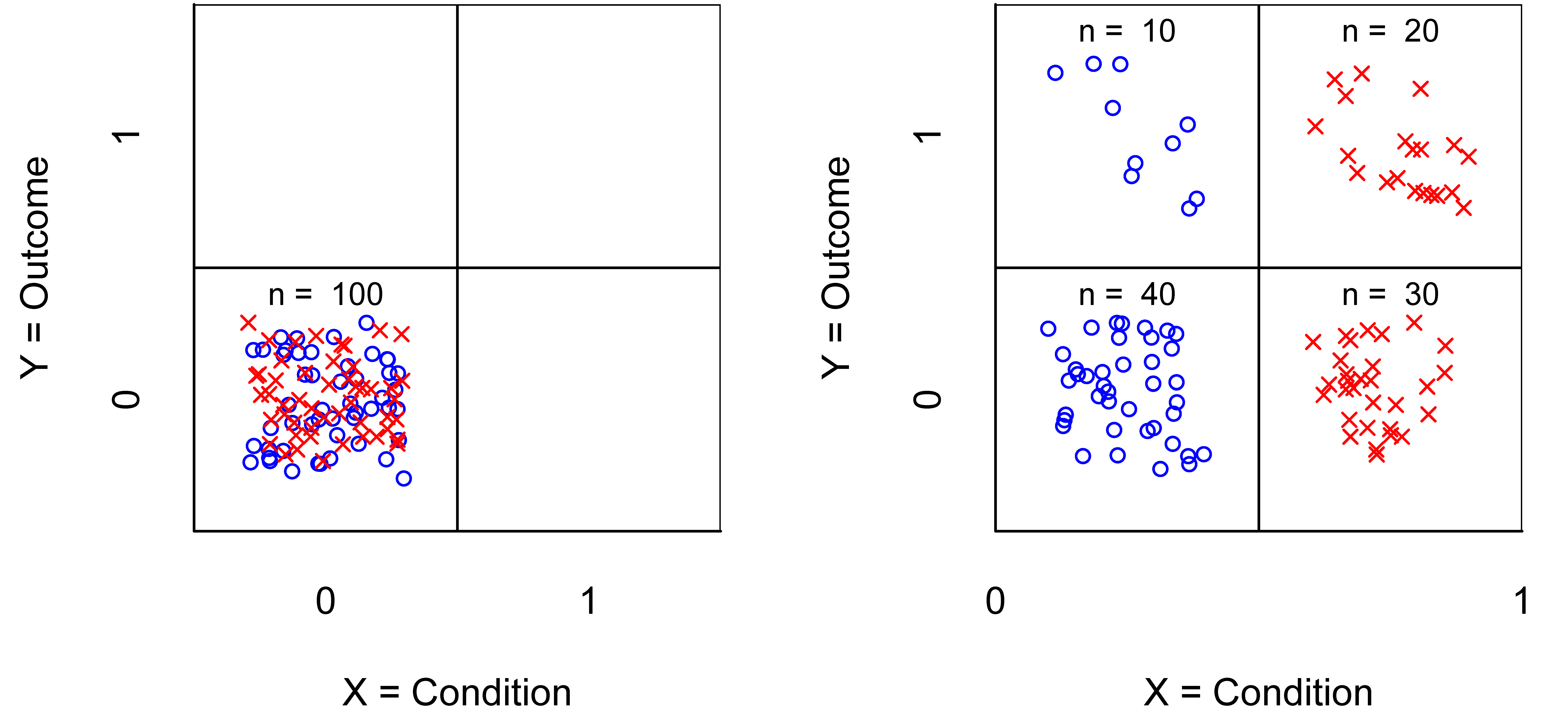
Figure F.1: \(XY\)-plot of the traditional experiment before (Left) and after (Right) manipulation. \(X\) = Condition (0 = no; 1 = yes); \(Y\) = Outcome (0 = no; 1 = yes). = control group; × = treatment group.
With a traditional RCT experiment, after the treatment usually all four corners have cases. In this example, 10 cases from the control group have moved from corner 3 to corner 2, suggesting a time effect. The cases from the treatment group have all moved to \(X\) = 1 (corner 2 or 4). Treatment and time had no effect on the 30 cases in corner 4. Treatment and time did have an effect on the 20 cases in corner 2. The data pattern in the four corners suggests that the treatment had an effect. There are more cases in corner 2 (resulting from a time effect and a treatment effect) than in corner 1. The odds ratio is an estimate of the average treatment effect: \((20/30)/(10/40) = 2.67\). Since the odds ratio is greater than 1, the conclusion is that \(X\) has a probabilistic sufficiency effect on \(Y\).124
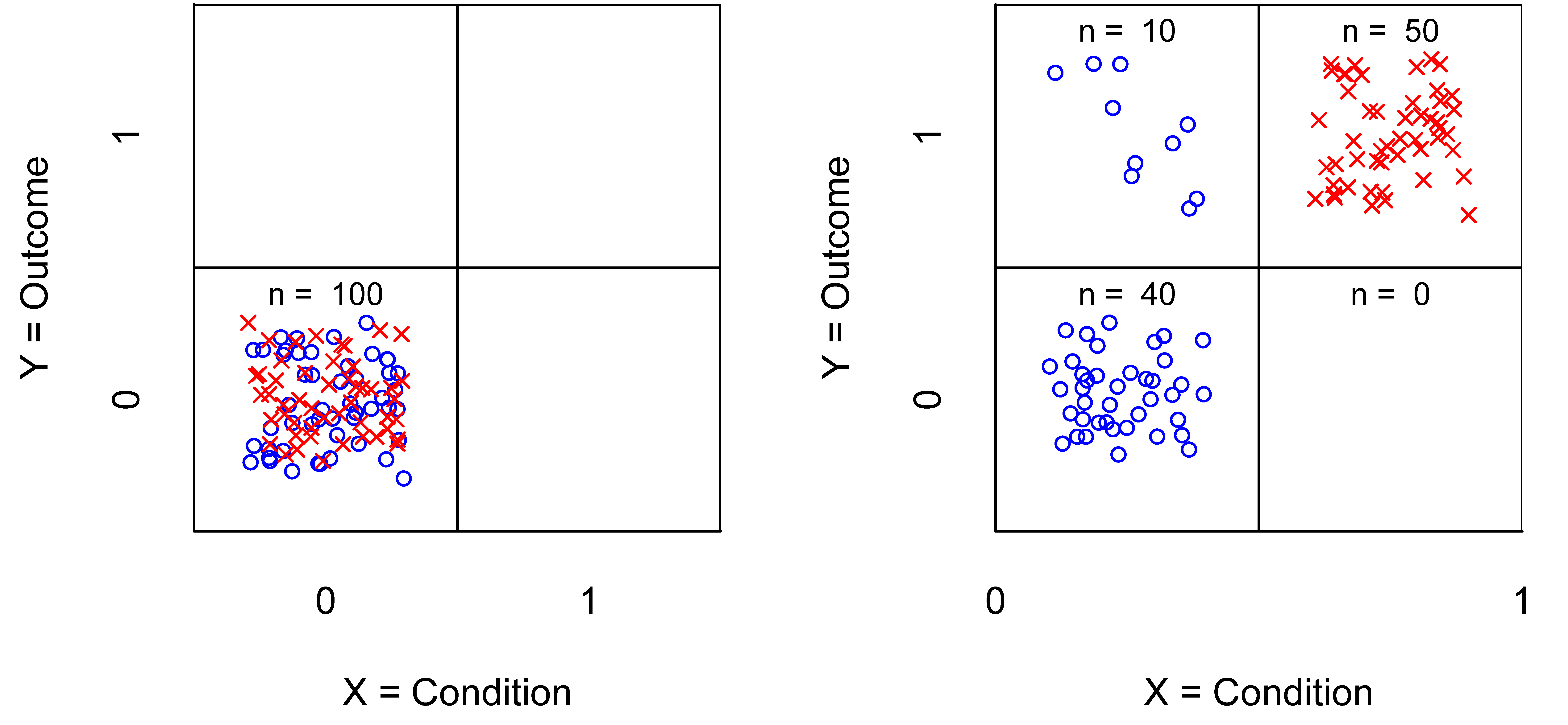
Figure F.2: \(XY\)-table of the sufficiency experiment before (Left) and after (Right) manipulation. \(X\) = Condition (0 = no; 1 = yes); \(Y\) = Outcome (0 = no; 1 = yes). = control group; × = treatment group.
F.2 Necessity lessons from the traditional experiment
Referring to Figures F.1-right and F.2-right, the (probabilistic) sufficiency experiments shows non-emptiness in corner 1 due to time effects. The non-emptiness reflects non-necessity. If \(X\) were necessary for \(Y\), this corner would remain empty after the manipulation. If this corner has cases, it can be concluded that the condition \(X = 1\) is not necessary for the effect \(Y = 1\), because the effect is possible without the condition. If this corner remains empty, necessity is not rejected. This ‘non-necessity test’, as part of a (probabilistic) sufficiency experiment, can only be done with the control group. The treatment group cannot be used for testing necessity because it cannot test the emptiness of corner 1. The non-necessity test with the control group is not a necessity experiment since no manipulation is involved in necessity testing. It can be understood as an observational study embedded in an experiment (or even as a longitudinal study because \(x\)- and \(y\)-scores are observed for two time points: before and after the manipulation).
The mathematical formula for the odds ratio is \(OR = \frac{c2 / c4}{c1 / c3} = \frac{c2 \cdot c3}{c1 \cdot c4}\) where \(c1\), \(c2\), \(c3\), and \(c4\) refer to the number of cases in corner 1, corner 2, corner 3, and corner 4, respectively. \(c2\) is the number of cases in the treatment group with outcome success, \(c4\) is the number of cases in the treatment group with outcome failure, \(c1\) is the number of cases in the control group with outcome success (spontaneous success), and \(c3\) is the number of cases in the control group with outcome failure. A value of \(OR > 1\) indicates that the condition \(X\) is associated with a higher likelihood of \(Y\), suggesting that \(X\) may be probabilistically sufficient to produce \(Y\).↩︎
The sufficiency experiment can be considered the deterministic version of the traditional experiment, namely when after the manipulation (Figure F.2), all cases of the treatment group are in corner 2. Then the odds ratio for estimating the average effect is infinite, regardless of the distribution of the cases in the control group: \((50/0)/(10/40) = \infty\). Note that this situation is named ‘perfect separation’ and is considered a problem for average effect statistical analysis. In this situation \(X\) is called a ‘perfect predictor’, which is considered a statistical problem.↩︎