4 Mathematics

4.1 Summary of this chapter

This chapter describes the mathematics of a necessity relationship between a pair of variables: $X$ is necessary for $Y$. The chapter focuses on necessity-in-degree (NiD) that describes the general situation of two continuous variables with an empty space in the upper-left corner of the $XY$-plot. Using a conventional Euclidean coordinate system where the $X$-axis runs horizontally with increasing values from left to right, and the $Y$-axis runs vertically with increasing values from bottom to top, this indicates that a high level of $X$ is necessary for a high level of $Y$. The mathematical approach described here can be extended to situations with dichotomous or discrete variables, or to analyzing other corners, though this is not addressed in this chapter. The chapter first presents the branches of mathematics applied in NCA (Section 4.2). In the subsequent section NCA’s mathematical model specification is presented (Section 4.3). It includes the specification of the bounding box, the ceiling line, and the model’s degrees of freedom. This is followed by a discussion on how to estimate a necessity model by estimating parameters related to the necessity effect size and model fit. Next, the situation of multiple necessary conditions is discussed, explaining why NCA considers multiple $X_jY$-planes (multiple projections), rather than one multidimensional space, and explaining how a chain of necessity can be analyzed (Section 4.6).

4.2 Branches of mathematics

Rather than relying on statistics and probability theory, NCA employs two branches of mathematics: geometry and algebra. Geometry describes relationships between objects and spaces including points, lines, angles, and planes. NCA focuses on points in the two-dimensional space ($XY$-plane), describes relationships between points (e.g., ceiling line) and considers the size of an area (e.g., effect size). Algebra uses symbols, letters, and numbers and describes their relationships and operations including variables, constants, functions, equations, and inequalities. NCA uses functions to describe the ceiling line with constants and variables, uses equations to calculate effect size, and uses inequalities to specify (in)feasible areas. When describing NCA, geometry and algebra are intertwined. NCA is not a statistical data analysis method per se, although it uses tools from statistics (Chapter 5).

4.3 Model specification

In NCA, variables $X$ and $Y$ can be dichotomous (two possible levels), discrete (more than two possible levels) or continuous variables (infinite number of possible levels). With numeric variables (including ratio- and interval-scale variables), effect size and other necessity parameters can be calculated. With categorical variables, these calculations are not possible unless equal distances between ordered categories are assumed (e.g., “low”, “medium”, “high”). NCA can handle both non-random and random variables. When NCA uses random variables for $X$ and $Y$, NCA only assumes that the univariate distributions are bounded, but no assumption is needed about the shape of the distribution.²⁹

NCA’s model specification consists of specifying the bounding box and the ceiling line.

4.3.1 Bounding box

NCA assumes that the condition and the outcome are bounded. There are two reasons for this. First, variables represent properties of phenomena. Many properties are finite, represented by minimum and maximum values of the variables, rather than being infinite (e.g., height of people). Second, the assumption that $X$ and $Y$ are bounded allows the definition and calculation of the necessity effect size (Section 4.4.1) and other NCA parameters (Sections 4.4.2 and 4.5). Assuming bounds on $(X,Y)$ means that there are four constants that define the ranges of the condition $X$ and the outcome $Y$:

\[\begin{equation} \tag{4.1} x_{\min} \leq x \leq x_{\max}\quad \text{ and } \quad y_{\min} \leq y \leq y_{\max} \end{equation}\]

These bounds define the bounding box in an $XY$-plot. The bounding box is defined by the minimum and maximum values of $X$ and $Y$, that is $[x_{\min}, x_{\max}] \times [y_{\min}, y_{\max}]$. The feasible and empty areas, as well as the ceiling line and its extensions, are defined relative to this bounding box.

The scope ($S$) is the area of the bounding box and is mathematically expressed as:

\[\begin{equation} \tag{4.2} S = {(x_{\max} - x_{\min})}\cdot{(y_{\max} - y_{\min})} \end{equation}\]

The bounding box can be constructed in two ways: theoretically and empirically. The theoretical scope is defined by theoretical bounds of $X$ and $Y$ when the theoretical bounds are known or presumed.³⁰ The empirical scope is defined by the observed minimum and maximum values of $X$ and $Y$. This option is often selected when theoretical bounds are unknown.

Without loss of generality (for the purpose of NCA), the variables can be linearly transformed to the unit box $[0,1]\times[0,1]$ to obtain a scope value of 1 (Section 8.5.2).³¹ Then a point $(x,y)$ gets transformed by min-max normalization into $(x',y')$ as follows:

\[\begin{equation} \tag{4.3} x' = \frac{x - x_{\min}}{x_{\max} - x_{\min}} \quad \text{ and } \quad y' = \frac{y - y_{\min}}{y_{\max} - y_{\min}} \end{equation}\]

4.3.2 Ceiling line

When necessity exists, the bounding box has an area where points are possible (feasible area) and an area where points are impossible (empty space or ceiling zone). The ceiling line³² is a line within the bounding box that separates these two areas. Specifying the ceiling line involves choosing its location (in which corner) and its form.

The location depends on the direction of the hypothesis (Section 3.5), which defines the expected empty corner. For a high-high hypothesis (presence/high value of $X$ is necessary for presence/high value of $Y$), the expected empty corner is the upper-left corner of the $XY$-plot (corner 1).³³

To specify the form of the ceiling line, several options exist. Figure 4.1 shows three classes of non-decreasing ceiling lines in a bounding box. The first class is the Ceiling Envelopment Free Disposal Hull (CE-FDH), which is a stepwise linear ceiling line consisting of several horizontal and vertical line segments (Figure 4.1-top-left), the second class is Ceiling Envelopment Variable Returns to Scale (CE-VRS), which is a concave piecewise linear ceiling consisting of several oblique line segments (Figure 4.1-top-right), and the final one is a linear ceiling line consisting of one segment (Figure 4.1-bottom). The ceiling line represents an upper bound on the outcome in the feasible area (the gray area). The ceiling line is considered a part of the feasible area.

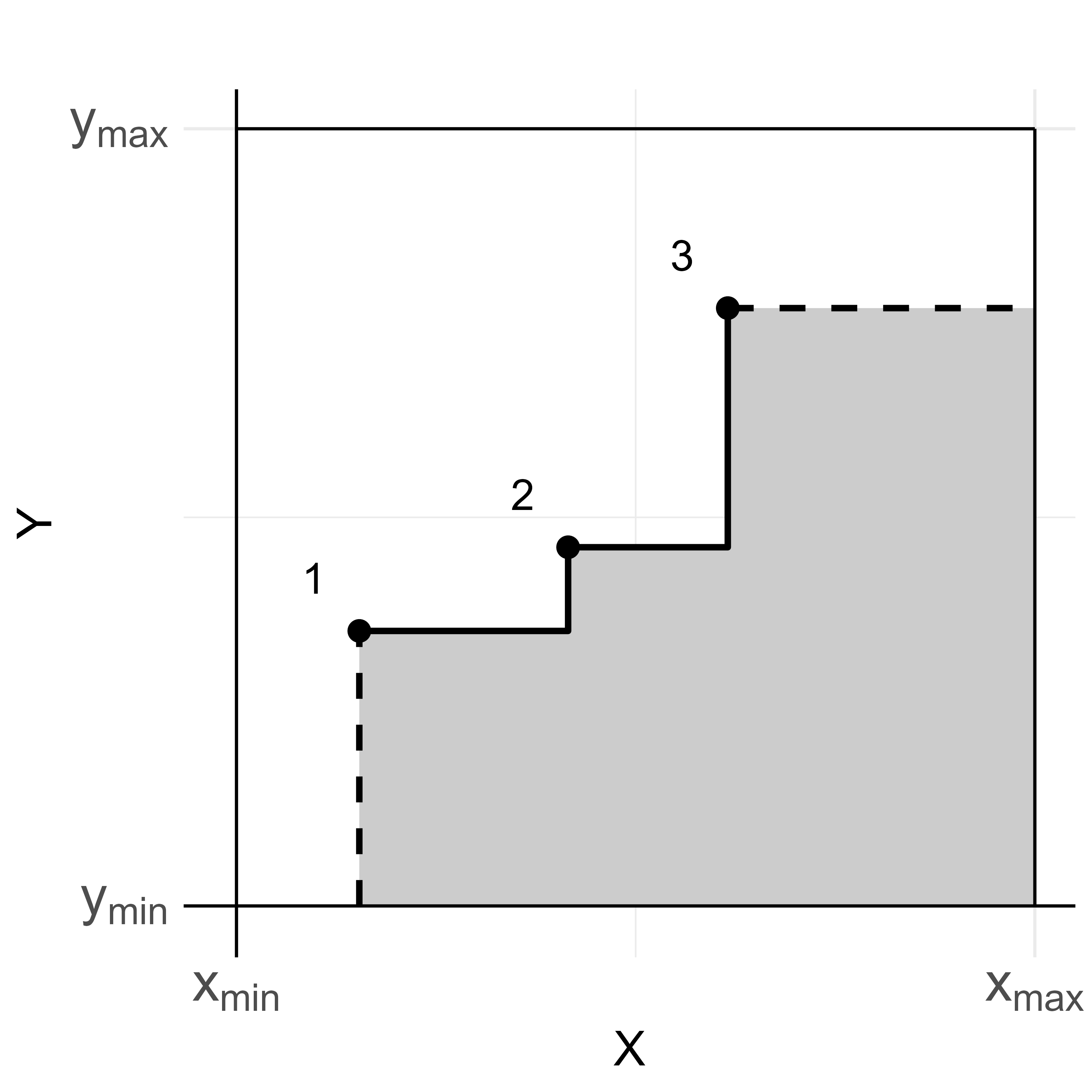
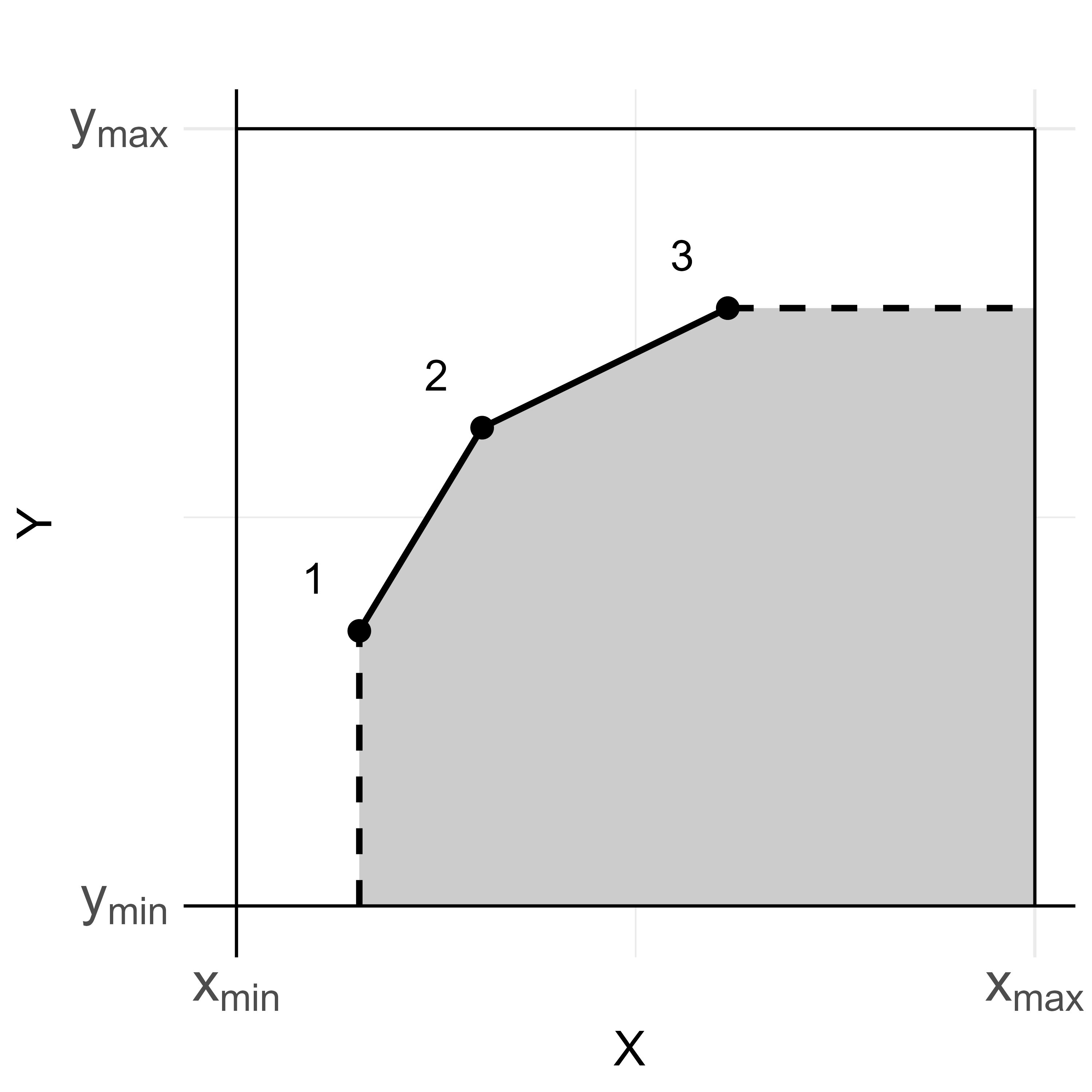
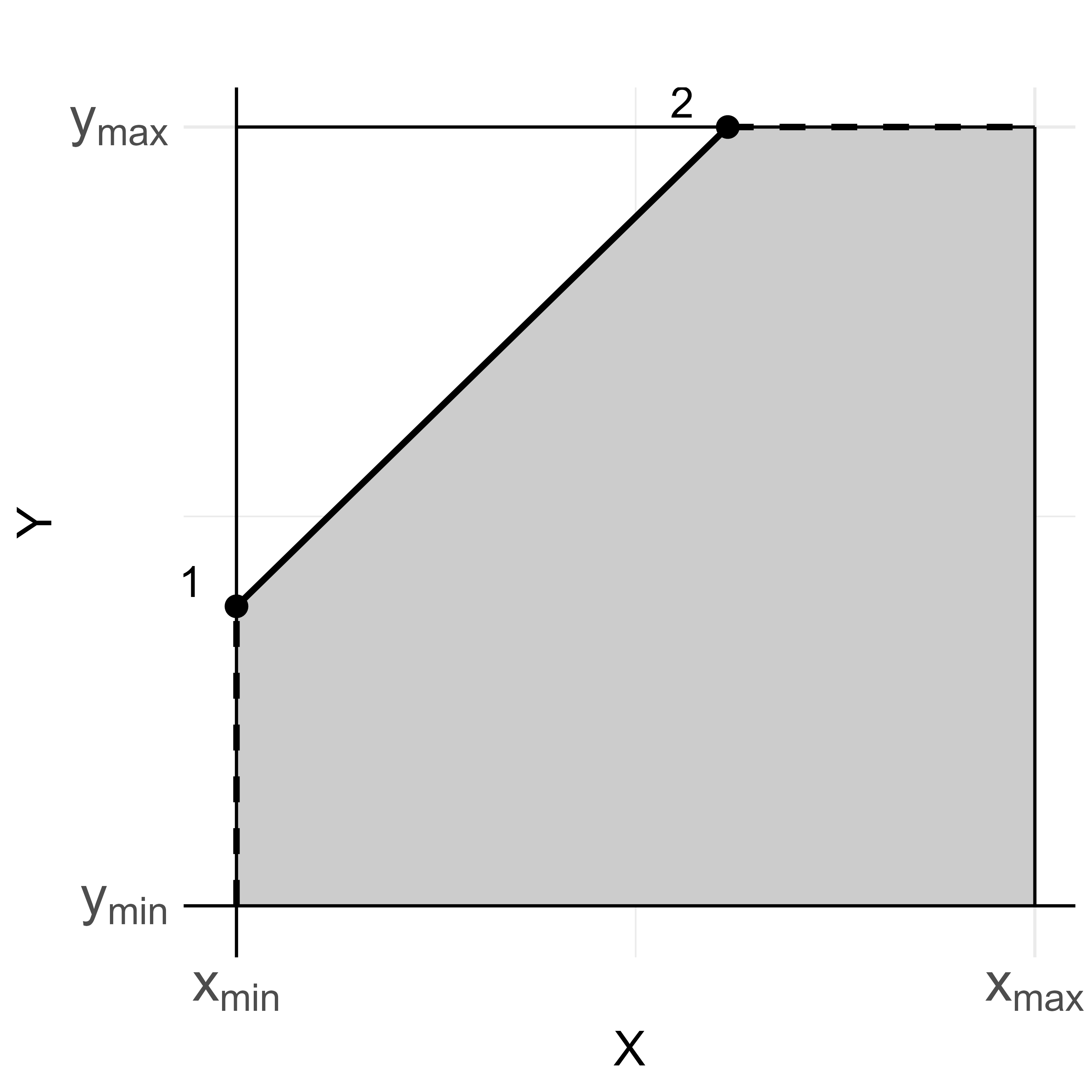
Three classes of ceiling lines within a bounding box for high-high necessity. Top-Left: stepwise linear. Top-Right: concave piecewise linear. Bottom: linear. White: ceiling zone. Gray: feasible area. Numbered points are peers (dominant point with no cases above and to the left of it) connected by solid line segments constructing the ceiling line. The dashed lines are extensions such that the ceiling line envelopes the feasible area.

Figure 4.1: Three classes of ceiling lines within a bounding box for high-high necessity. Top-Left: stepwise linear. Top-Right: concave piecewise linear. Bottom: linear. White: ceiling zone. Gray: feasible area. Numbered points are peers (dominant point with no cases above and to the left of it) connected by solid line segments constructing the ceiling line. The dashed lines are extensions such that the ceiling line envelopes the feasible area.

A ceiling line is assumed to be non-decreasing for two reasons.³⁴ First, it allows the expression that at least a certain level of $X$ is necessary for a certain level of $Y$. Second, a non-decreasing ceiling line has the ‘no-reversal’ (no change of direction) property. This means that if a point $(x,y)$ is in the ceiling zone, then any point $(x',y')$ to the left or above it (a point with $x'\leq x$ and $y'\geq y$) and within the bounding box is also in the ceiling zone. Similarly, if a point $(x,y)$ is in the feasible area, then any point $(x',y')$ in the bounding box with $x' \geq x$ and $y' \leq y$ is also in the feasible area. This property is used for the mathematical expression of the ceiling line (see below) and for two measures of imperfect necessity, namely purity and solidity (Sections 4.5.4 and 4.5.5, respectively).

4.3.2.1 Stepwise linear ceiling line

NCA uses the stepwise linear ceiling line (CE-FDH) as the base ceiling model. It refers to the Free Disposal Hull (FDH) technique (Deprins et al., 1984) that originates in production economics. This application of FDH identifies the efficiency of decision-making units (DMUs) with a certain production input ($X$) and output ($Y$). The technique assumes the free disposability property meaning that if a DMU can produce a certain output, it can also reduce the amount of output without using additional input, and use more input without increasing output. FDH identifies the most efficient DMUs (points with maximum output for a given input and minimum input for a given output). The outer boundary of the hull (‘envelope’ or ‘frontier’) connects the most efficient points (called ‘peers’). Points below the frontier are considered inefficient.

NCA uses the FDH technique in 2D. In NCA’s context, the hull is called the feasible area, and the disposability property is called the no-reversal property. The feasible area is the smallest area defined by peers: a strictly increasing set of points, $(x_i,y_i)_{i=1,\ldots,P}$ for which

\[\begin{equation} \tag{4.4} x_i<x_{i+1}\quad\text{and}\quad y_i<y_{i+1}\quad\text{for}\quad i=1,\ldots,P-1 \end{equation}\]

Where $P$ is the number of peers. Peers are points that dominate other points. When the upper-left corner is the expected empty corner (as in Figure 4.1), no points exist to the left and above the peers.

A class of ceiling lines is defined by the way that peers are defined and connected. The CE-FDH-class of ceiling lines consists of all models with a feasible area generated by a set of $P$ peers connected by horizontal and vertical line segments (Figure 4.1-top-left).

Let the peers be $(x_i,y_i)_{i=1,\ldots,P}$. The feasible space generated by these peers is the hypograph³⁵ of the ceiling function $f(x)$, defined for $x\in[x_1,x_{\max}]$ by

\[\begin{equation} \tag{4.5} f_{\mathrm{CE-FDH}}(x)= \begin{cases} y_i & \text{if } x_i\le x<x_{i+1}\quad (i=1,\ldots,P-1),\\ y_P & \text{if } x_P\le x\le x_{\max} \end{cases} \end{equation}\]

and $f_{\mathrm{CE-FDH}}(x)$ is not defined for $x<x_1$.

The generalized inverse is:

\[\begin{equation} \tag{4.6} \begin{aligned} f_{\mathrm{CE-FDH}}^{-}(y) &= \inf\{x\mid f_{\mathrm{CE-FDH}}(x)\ge y\}\\ &= \begin{cases} x_1 & \text{if } y\le y_1,\\ x_{i+1} & \text{if } y_i<y\le y_{i+1}\quad (i=1,\ldots,P-1) \end{cases} \end{aligned} \end{equation}\]

and $f_{\mathrm{CE-FDH}}^{-}(y)$ is undefined (infeasible) if $y>y_P$.

The associated feasible space is generated by all points on the line segments from $(x_i,y_i)$ to $(x_{i+1},y_{i+1})$ for $i=1,\ldots,P-1$.

The ceiling line is given by the sequence of line segments from $(x_1,y_{\min})$ to $(x_1,y_1)$, to $(x_2,y_1)$, to $(x_2,y_2)$, and so on, ending at $(x_P,y_P)$ and $(x_{\max},y_P)$. Possibly, the first segment from $(x_1,y_{\min})$ to $(x_1,y_1)$ and/or the last segment from $(x_P,y_P)$ to $(x_{\max},y_P)$ has length equal to zero (starts and ends at the bounding box). When the first peer starts at $x = x_{min}$ and the last peer ends at $y = y_{max}$ the bounding box is called a tight bounding box.

4.3.2.2 Concave piecewise linear (CE-VRS) ceiling line

The CE-VRS-class of ceiling line consists of all models with a set of $P$ peers such that the sequence of peers forms a concave sequence, i.e., the slopes between consecutive peers strictly decrease:

\[\begin{equation} \tag{4.7} \frac{y_{i+1}-y_i}{x_{i+1}-x_i} > \frac{y_{i+2}-y_{i+1}}{x_{i+2}-x_{i+1}} \quad\text{for}\quad i=1,\ldots,P-2 \end{equation}\]

The ceiling function is given by linear interpolation between consecutive peers:

\[\begin{equation} \tag{4.8} f_{\mathrm{CE-VRS}}(x)=y_{i-1}+\frac{y_i-y_{i-1}}{x_i-x_{i-1}}(x-x_{i-1}) \quad\text{if}\quad x_{i-1}\le x\le x_i\quad (i=2,\ldots,P) \end{equation}\]

and $f_{\mathrm{CE-VRS}}(x)=y_P$ if $x\ge x_P$, while $f_{\mathrm{CE-VRS}}(x)$ is not defined for $x<x_1$.

The generalized inverse is:

\[\begin{equation} \tag{4.9} \begin{aligned} f_{\mathrm{CE-VRS}}^{-}(y) &= \inf\{x\mid f_{\mathrm{CE-VRS}}(x)\ge y\}\\ &= \begin{cases} x_1 & \text{if } y\le y_1,\\[2mm] x_i+\dfrac{x_{i+1}-x_i}{y_{i+1}-y_i}(y-y_i) & \text{if } y_i<y\le y_{i+1}\\ & \quad (i=1,\ldots,P-1) \end{cases} \end{aligned} \end{equation}\]

and $f_{\mathrm{CE-VRS}}^{-}(y)$ is undefined (infeasible) if $y>y_P$.

The associated feasible space is generated by all points on the line segments from $(x_i,y_i)$ to $(x_{i+1},y_{i+1})$ for $i=1,\ldots,P-1$.

The ceiling line follows the linear segments from $(x_1,y_{\min})$ to $(x_1,y_1)$, then to $(x_2,y_2)$, and so on, ending at $(x_P,y_P)$ and $(x_{\max},y_P)$. Possibly, the first and/or last segment has length equal to zero.

4.3.2.3 Linear ceiling line

The class of linear ceiling lines consists of models with a ceiling that is a (positive-length) segment of a line. The ceiling function is

\[\begin{equation} \tag{4.10} f_{\mathrm{LIN}}(x)=\max\{y_{\min},\min\{y_{\max},a+bx\}\} \end{equation}\]

with $b>0$ to ensure the line is strictly increasing and with $(a+bx_{\min},\,a+bx_{\max}]\cap[y_{\min},y_{\max}]$ to ensure the line intersects the bounding box with a segment of positive length. This is equivalent to

\[\begin{equation} \tag{4.11} a+bx_{\max}>y_{\min}\quad\text{and}\quad a+bx_{\min}<y_{\max} \end{equation}\]

which in turn is equivalent to

\[\begin{equation} \tag{4.12} y_{\min}-bx_{\max}<a<y_{\max}-bx_{\min}. \end{equation}\]

The line $y=a+bx$ intersects the boundary of the bounding box in two points $(x_1,y_1)$ and $(x_2,y_2)$ with

\[\begin{equation} \tag{4.13} (x_1,y_1)=\big(\max\{x_{\min},(y_{\min}-a)/b\},\ \max\{y_{\min},a+bx_{\min}\}\big) \end{equation}\]

and

\[\begin{equation} \tag{4.14} (x_2,y_2)=\big(\min\{x_{\max},(y_{\max}-a)/b\},\ \min\{y_{\max},a+bx_{\max}\}\big). \end{equation}\]

The set of two points $(x_1,y_1)$ and $(x_2,y_2)$ forms a set of peers. In terms of these peers, the ceiling can be written as

\[\begin{equation} \tag{4.15} f_{\mathrm{LIN}}(x)= \begin{cases} y_1+\dfrac{y_2-y_1}{x_2-x_1}(x-x_1)=a+bx & \text{if } x_1\le x\le x_2,\\ y_2 & \text{if } x\ge x_2 \end{cases} \end{equation}\]

with $f_{\mathrm{LIN}}(x)$ not defined for $x<x_1$.

The generalized inverse is:

\[\begin{equation} \tag{4.16} \begin{aligned} f_{\mathrm{LIN}}^{-}(y)=\inf\{x\mid f_{\mathrm{LIN}}(x)\ge y\}\\ &= \begin{cases} x_1 & \text{if } y\le y_1,\\[2mm] x_1+\dfrac{x_2-x_1}{y_2-y_1}(y-y_1)=\dfrac{y-a}{b} & \text{if } y_1<y\le y_2\\ \end{cases} \end{aligned} \end{equation}\]

and $f_{\mathrm{LIN}}^{-}(y)$ is undefined (infeasible) if $y>y_2$.

The ceiling line consists of the line segments from $(x_1,y_{\min})$ to $(x_1,y_1)$, then to $(x_2,y_2)$, and finally to $(x_{\max},y_2)$. Possibly, the first and/or last segment has length equal to zero.

4.3.3 Model degrees of freedom

A necessity model specifies the bounding box with the ceiling line that is inside it. The ceiling line is assumed not to be outside the bounding box. Model degrees of freedom refers to the minimum number of parameters that are needed to describe the necessity model. The bounding box has $4$ degrees of freedom. It can be described by, for example, the coordinates of the lower-left and the upper-right corner points: $x_{\min}, y_{\min}, x_{\max}, y_{\max}$.

Since a sequence of peers in the two classes of segmented ceiling lines (CE-FDH and CE-VRS) is defined in terms of strict inequalities, each peer can change position slightly without violating the conditions. Hence, the degrees of freedom of each of the CE-FDH and CE-VRS classes is $2P$.

Since the class of linear ceiling lines only imposes restrictions on $a$ and $b$ through strict inequalities, the degrees of freedom equals $2$.

Therefore the general expression for the degrees of freedom of a necessity model is:

\[\begin{equation} \tag{4.17} df_{\text{model}} = \begin{cases} 6, & \text{linear ceiling line}. \\ 2P + 4, & \text{segmented ceiling line}. \end{cases} \end{equation}\]

where $P$ is the number of peers of the segmented ceiling lines (CE-FDH and CE-VRS).

4.4 Mathematical estimation

Mathematical estimation techniques using different ceiling lines. CE-FDH: stepwise linear ceiling line. CR-FDH: linear ceiling line (shown as the lower solid line). C-LP: linear ceiling line (shown as dashed line). CE-VRS: concave piecewise linear ceiling line (shown as segments passing through A, B, C, D, and E). CR-VRS: linear ceiling line (shown as the upper solid line). QR (Quantile Regression): linear ceiling line (shown as the dashed-dotted line in the middle). Population ceiling line: Y = 0.3 + X. Population effect size = 0.25. 50 points randomly selected from the population.

Figure 4.2: Mathematical estimation techniques using different ceiling lines. CE-FDH: stepwise linear ceiling line. CR-FDH: linear ceiling line (shown as the lower solid line). C-LP: linear ceiling line (shown as dashed line). CE-VRS: concave piecewise linear ceiling line (shown as segments passing through A, B, C, D, and E). CR-VRS: linear ceiling line (shown as the upper solid line). QR (Quantile Regression): linear ceiling line (shown as the dashed-dotted line in the middle). Population ceiling line: Y = 0.3 + X. Population effect size = 0.25. 50 points randomly selected from the population.

The mathematical estimation of the necessity model consists of estimating the parameters of the bounding box and the ceiling line from data. This can be done with the NCA software (Appendix B).

The estimation of the bounding box requires that the analyst selects the type of bounding box (defined by the theoretical or empirical scope). For the theoretical scope, the analyst specifies $x_{min}$, $y_{min}$, $x_{max}$ and $y_{max}$. For the empirical scope the software estimates these values by taking the observed extremes.

The estimation of the ceiling line requires that the analyst selects the form of the ceiling line. If a segmented ceiling line is selected (CE-FDH or CE-VRS), the software provides the estimated $x$- and $y$-coordinates of the peers. To select a linear ceiling line there are several options. The Ceiling Regression Free Disposal Hull ceiling line (CR-FDH) is a trend line through the CE-FDH peers using least squares optimization. The Ceiling Regression Variable Returns to Scale (CR-VRS) ceiling line is the trend line through the CE-VRS peers using least squares optimization. The Ceiling - Linear Programming (C-LP) ceiling line is the line that is tight to the CE-FDH peers such that the sum of heights of the CE-FDH peers is minimized (“least sum”). The different lines are shown in Figure 4.2.³⁶

After selecting the form of the line, the software provides the values of the parameters to describe the ceiling line (e.g., intercept and slope for the linear ceiling line). Criteria for selecting the type of bounding box and form of the ceiling line are discussed in Section 9.3.

NCA’s mathematical estimations with the above ceiling techniques are based on the location of the peers. CE-FDH and CE-VRS use peers directly, while the linear ceiling lines CR-FDH, CR-VRS and C-LP ceiling line use them indirectly. The use of only points near the border is motivated by several fundamental considerations.³⁷ First, NCA’s primary object of interest is the empty space above the ceiling: the region where observations are impossible. This follows necessity logic: if not $X$, then not $Y$. The ceiling zone is the complement of the feasible area in the bounding box. NCA quantifies the size of this zone and relates it to the size of the bounding box, which requires knowing the maximum feasible area but does not require modeling how points are distributed within that feasible area. Consequently, only points close to the ceiling are informative for locating the boundary. Points far below it do not contribute to identifying the boundary.

Second, conceptually, in NCA’s deterministic logic, the ceiling is an abrupt transition from a region that can contain points to a region that cannot, more like a cliff edge than a gradual slope. The characteristic feature of a ceiling is thus a sharp boundary between feasibility and infeasibility. Methods that estimate the ceiling indirectly via a gradual (non-abrupt) distributional model of all data risk misrepresenting this discontinuity. A gradual model can blur the boundary and thereby estimate a “soft” transition that is not characteristic of a true ceiling.

Third, ceiling estimates should be insensitive to data far below the ceiling. For example, increasing the density of points in the lower-right corner should not have an effect on how the ceiling is constructed. Such points would pull the estimated ceiling estimates downward. This inflates the estimated empty space and thus overstates the true effect size. For this reason, ceiling estimation techniques that rely on fitting the full distribution under the ceiling are generally risky and should be applied with caution.³⁸ This is illustrated with the distribution-based Quantile Regression (QR) ceiling line. In Figure 4.2, this line lies among the other ceilings (that all only use points near the ceiling) and approximates the true ceiling line well. However, after altering the distribution of points by adding observations in the lower-right corner, the QR-based ceiling becomes biased, whereas ceilings estimated from on upper points remain stable (4.3). Broader evidence from Monte Carlo simulations likewise suggests that a distribution-based method like QR can exhibit bias, even at larger sample sizes, warranting prudence in their use (Section 5.5).

Comparison of an estimation techniques based on the distribution of all data below the ceiling: QR = Quantile Regression (shown as the near-horizontal dash-dotted line) and based on upper peers (the other lines). Population ceiling line = $Y = 0.3 + X$. Population effect size is 0.25. First 50 points randomly selected from the population, next 50 points added in the lower-right corner.

Figure 4.3: Comparison of an estimation techniques based on the distribution of all data below the ceiling: QR = Quantile Regression (shown as the near-horizontal dash-dotted line) and based on upper peers (the other lines). Population ceiling line = $Y = 0.3 + X$. Population effect size is 0.25. First 50 points randomly selected from the population, next 50 points added in the lower-right corner.

4.4.1 Effect size

When a high value of $X$ is necessary for a high value of $Y$, the ceiling line determines the maximum possible $y$-value ($y$ = $y_{c}$) for a given $x$-value, while the bounding box determines the absolute maximum possible $y$-value ($y=y_{\max}$). The difference between the two can be considered the constraint that $X$ puts on $Y$. The increase of the ceiling line expresses the change in constraint under varying values of $X$. The maximum constraint occurs for $x = x_{\min}$. The effect builds up with increasing $x$ at a rate determined by the increase in the ceiling line. The total effect is then the area between the ceiling line and the maximum possible $y = y_{\max}$.

Referring to Figure 4.1, the general expression for the necessity effect size is as follows. Let the bounding box be $B=[x_{\min},x_{\max}]\times[y_{\min},y_{\max}]$ with $x_{\max}>x_{\min}$ and $y_{\max}>y_{\min}$ and let $c(x)$ be the ceiling value of defined on $[x_1,x_{\max}]$ (with $x_1$ the leftmost $x$ where the ceiling is defined).

The scope $S$ is the area of the bounding box:

\[\begin{equation} \tag{4.22} S=(x_{\max}-x_{\min})(y_{\max}-y_{\min}) \end{equation}\]

The feasible area is the area under the ceiling line $f(x)$ (only for $x\in[x_1,x_{\max}]$):

\[\begin{equation} \tag{4.23} F=\int_{x_1}^{x_{\max}}\big(f(x)-y_{\min}\big)\,dx \end{equation}\]

The ceiling zone $C$ is the complement of the feasible area within the bounding box:

\[\begin{equation} \tag{4.27} C=S-F \end{equation}\]

Equivalently, $C$ can be written as the sum of the left strip (where the ceiling is undefined) and the area above the ceiling for $x\in[x_1,x_{\max}]$:

\[\begin{equation} \tag{4.25} C=(x_1-x_{\min})(y_{\max}-y_{\min})+\int_{x_1}^{x_{\max}}\big(y_{\max}-f(x)\big)\,dx \end{equation}\]

Consequently the effect size $d$ is:

\[\begin{equation} \tag{4.26} \begin{aligned} d &= \frac{C}{S}\\ &= 1-\frac{F}{S} \end{aligned} \end{equation}\]

The effect size for the different ceiling classes can be derived from the ceiling line equations.

4.4.1.1 Class of stepwise linear ceiling lines

For the CE-FDH class of ceiling line, see Equation (4.5), the feasible area is:

\[\begin{equation} \tag{4.29} F_{\mathrm{CE-FDH}} =\sum_{i=1}^{P-1}(x_{i+1}-x_i)(y_i-y_{\min}) +(x_{\max}-x_P)(y_P-y_{\min}) \end{equation}\]

Therefore, the effect size is:

\[\begin{equation} \tag{4.30} \begin{aligned} d_{\mathrm{CE-FDH}} &= 1-\frac{F_{\mathrm{CE-FDH}}}{S}\\ &= 1-\frac{\sum_{i=1}^{P-1}(x_{i+1}-x_i)(y_i-y_{\min})+(x_{\max}-x_P)(y_P-y_{\min})}{(x_{\max}-x_{\min})(y_{\max}-y_{\min})} \end{aligned} \end{equation}\]

4.4.1.2 Class of concave piecewise linear ceiling lines

For the CE-VRS class of ceiling line, see Equation (4.8), the feasible area is:

\[\begin{equation} \tag{4.31} F_{\mathrm{CE-VRS}} =\sum_{i=1}^{P-1}(x_{i+1}-x_i)\left(\frac{y_i+y_{i+1}}{2}-y_{\min}\right) +(x_{\max}-x_P)(y_P-y_{\min}) \end{equation}\]

Therefore, the effect size is:

\[\begin{equation} \tag{4.32} \begin{aligned} d_{\mathrm{CE-VRS}} &= 1-\frac{F_{\mathrm{CE-VRS}}}{S}\\ &= 1-\frac{\sum_{i=1}^{P-1}(x_{i+1}-x_i)\left(\frac{y_i+y_{i+1}}{2}-y_{\min}\right)+(x_{\max}-x_P)(y_P-y_{\min})}{(x_{\max}-x_{\min})(y_{\max}-y_{\min})} \end{aligned} \end{equation}\]

4.4.1.3 Class of linear ceiling lines

For the class of linear ceiling line, see Equation (4.15), let the ceiling line intersect the bounding box at two points $(x_1,y_1)$ and $(x_2,y_2)$ with $x_{\min}\le x_1 < x_2 \le x_{\max}$. The feasible area under the ceiling within the bounding box is:

\[\begin{equation} \tag{4.33} \begin{aligned} F_{\mathrm{LIN}} &= (x_2-x_1)\left(\frac{y_1+y_2}{2}-y_{\min}\right)\\ &\quad +(x_{\max}-x_2)(y_{\max}-y_{\min}) \end{aligned} \end{equation}\]

Therefore, the effect size is: \[\begin{equation} \tag{4.34} \begin{aligned} d_{\mathrm{LIN}} &= 1-\frac{F_{\mathrm{LIN}}}{S}\\ &= 1-\frac{(x_2-x_1)\left(\tfrac{y_1+y_2}{2}-y_{\min}\right)+(x_{\max}-x_2)(y_{\max}-y_{\min})}{(x_{\max}-x_{\min})(y_{\max}-y_{\min})} \end{aligned} \end{equation}\]

4.4.2 Necessity inefficiency

As illustrated in Figure 4.4, for the standard case of a linear ceiling line above the diagonal, $X$ may not constrain $Y$ over the entire ranges of $X$ and $Y$ within the bounding box. The ceiling line intersects with the bounding box: $[x_{\min}, y_{\operatorname{cmin}}]$ and $[x_{\operatorname{cmax}}, y_{\max}]$. The vertical extension is the distance $y_{\operatorname{1}} - y_{\min}$, and the horizontal extension $x_{\max} - x_{\operatorname{2}}$.

$Necessity inefficiency refers to the part of the feasible area where $Y$ is not constrained by $X$ in the area $[x_{min}, x_{max}]\times[y_{min}, y_{1}]$ (outcome inefficiency), and to the part of the feasible area where $X$ does not constrain $Y$ in the area $[x_{2}, x_{max}] \times [y_{min}, y_{max}]$ (condition inefficiency).$

Figure 4.4: Necessity inefficiency refers to the part of the feasible area where $Y$ is not constrained by $X$ in the area $[x_{min}, x_{max}]\times[y_{min}, y_{1}]$ (outcome inefficiency), and to the part of the feasible area where $X$ does not constrain $Y$ in the area $[x_{2}, x_{max}] \times [y_{min}, y_{max}]$ (condition inefficiency).

When $(x_c,y_c)$ is a point on the ceiling line and $x < x_{c}$, then $x$ is a bottleneck for $y = y_{c}$. Only an increased value of $x$ such that $x\geq x_{c}$ enables a value $y = y_{c}$. For reaching the value of $y = y_{\max}$ it is necessary to have a value of $x\geq x_{\operatorname{2}}$, where $x_{\operatorname{2}}$ is the value of $x$ of the point where the ceiling line crosses the $y = y_{\max}$ line. Thus, for enabling the maximum possible value $y_{\max}$, $x$ should be at least $x = x_{\operatorname{2}}$. Increasing $x$ beyond $x = x_{\operatorname{2}}$ for enabling $y = y_{\max}$ is not needed as $y$ is no longer constrained. This is called ‘inefficiency’ regarding enabling the maximum outcome.

Condition inefficiency specifies the extent to which $x$ does not constrain $y$ for levels of $x_{\operatorname{2}}\leq x\leq x_{\max}$. Only for $x_{\min}\leq x\leq\ x_{\operatorname{2}}$, $x$ constrains $y$ (ceiling line exists for $x_{\min} \leq x\leq x_{\operatorname{2}}$). Condition inefficiency is expressed as a percentage:

\[\begin{equation} \tag{4.50} \text{condition inefficiency} = \frac{x_{\max} - x_{\operatorname{2}}}{x_{\max} - x_{\min}} * 100\% \end{equation}\]

where $x_{\max}$ and $x_{\min}$ are the minimum and maximum values of $x$ (bounds) and $x_{\operatorname{2}}$ is the value of $x$ of the point where the ceiling line crosses the $y = y_{\max}$ line.

Similarly, outcome inefficiency specifies the extent to which $Y$ is not constrained by $X$ for lower levels of $y_{\min}\leq y\leq y_{\operatorname{1}}$, where $y_{\operatorname{1}}$ is the value of $y$ of the point where the ceiling line crosses the $x = x_{\min}$ line. Only for $y_{\operatorname{1}}\leq y\leq y_{\max}$, $y$ is constrained by $X$ (ceiling line exists for $y_{\operatorname{1}}\leq y\leq y_{\max}$). Outcome inefficiency is expressed as a percentage:

\[\begin{equation} \tag{4.51} \text{outcome inefficiency} = \frac{y_{\operatorname{1}} - y_{\min}}{y_{\max} - y_{\min}} * 100\% \end{equation}\]

where $y_{\min}$ and $y_{\max}$ are the minimum and maximum values of $Y$ (bounds), and $y_{\operatorname{1}}$ is the value of $y$ of the point where the ceiling line crosses the $x = x_{\min}$ line. Outcome inefficiency is 0% if $X$ constrains $Y$ for all values of $Y$; outcome inefficiency is 100% if $Y$ is not constrained for any value of $X$.

4.5 Model fit

NCA’s mathematical model specification differs from a statistical model specification. The latter includes a random term called the error term or disturbance ($\varepsilon$) representing the variation in the data. NCA does not specify the distribution of data under the ceiling and therefore the model does not include the random term. Thus, NCA’s model consists of a bounding box with a ceiling line and is deterministic (possibly with noise and exceptions, see Section 4.5.4, not probabilistic).

Since NCA cannot rely on statistical (distribution-based) approaches for evaluating model fit, NCA-specific metrics of model fit are developed to quantify how well an NCA model captures the underlying necessity pattern in the data, and how closely the model’s predicted values match observed values. In this section eight metrics of model fit are presented: complexity, fit, ceiling accuracy, exceptions, noise, support, spread, and sharpness.

4.5.1 Complexity

The complexity metric ($cp$) can be used to balance parsimony against accuracy. A complex model fits data well (accuracy) but needs more parameters, whereas the model with low complexity is attractive for generalization and practical usefulness, but may lack accuracy.

The proposed complexity measure relates to the model degrees of freedom (Section 4.3.3). When the degrees of freedom for the bounding box are fixed at four, the model degrees of freedom depend only on the ceiling line. The ceiling line degrees of freedom equal the model degrees of freedom minus 4. That is:

\[\begin{equation} \tag{4.52} df_{\text{ceiling}} = \begin{cases} 2, & \text{linear ceiling line} \\ 2P, & \text{segmented ceiling line} \end{cases} \end{equation}\]

where $P$ is the number of peers on the piecewise linear ceiling as defined in Section 4.3.3.

The more degrees of freedom, the more complex the ceiling is. The linear ceiling line has the lowest complexity. This base level is set at 1 (degrees of freedom divided by 2) and represents 1 pair of parameters needed for describing a linear ceiling line (intercept, slope). The complexity of a segmented ceiling line can be described by the number of peers. Each peer can be described by 1 pair of parameters ($x$-coordinate and $y$-coordinate). Therefore, complexity is defined as:

\[\begin{equation} \tag{4.53} complexity_{\text{}} = \begin{cases} 1, & \text{linear ceiling line} \\ P, & \text{segmented ceiling line} \end{cases} \end{equation}\]

where $P$ is the number of peers.

4.5.2 Fit

The model fit metric fit ($ft$) compares a selected ceiling line with the CE-FDH ceiling line. CE-FDH follows the border closely and gives the maximum possible effect size under strict necessity (no cases above the ceiling). By definition, fit of CE-FDH equals 100%. For other selected ceiling lines, fit is usually lower. The fit metric indicates how closely the selected ceiling line follows the pattern of the boundary like the CE-FDH does.³⁹

Fit can be expressed as follows:

\[\begin{equation} \tag{4.55} fit = \begin{cases} \frac{d_{\text{ceiling}}}{d_{\text{CE-FDH}}} \times 100\% & \text{if } d_{\text{ceiling}} \leq d_{\text{CE-FDH}} \\ \text{undefined} & \text{if } d_{\text{ceiling}} > d_{\text{CE-FDH}} \end{cases} \end{equation}\]

where $d_{ceiling}$ is the effect size of the selected ceiling line and $d_{CE-FDH}$ is the effect size of the CE-FDH ceiling line. Fit is undefined when the effect size of the selected ceiling line exceeds that of the CE-FDH ceiling line, to avoid interpretational issues.

4.5.3 Ceiling accuracy

Model fit metric ceiling accuracy ($ca$) refers to the emptiness of the ceiling zone. It quantifies the degree to which the expected empty corner is indeed empty. A selected ceiling line defines the ceiling zone. With a strict interpretation of necessity, the ceiling zone should not have points, and all points should be in the feasible area. Figure 4.5-left shows an example of two points being in the ceiling zone. The presence of points in the ceiling zone may have several explanations. First, the point can be an observation (case) from an empirical study with measurement error or sampling error (Section 9.8). Second, the selected ceiling line may be too low, resulting in points above it.⁴⁰ Third, from the typicality perspective of necessity (Section 2.4.3), the point might represent a rare permissible exception, transforming the expression ‘$X$ is always necessary for $Y$’ into ‘$X$ is typically necessary for $Y$’.

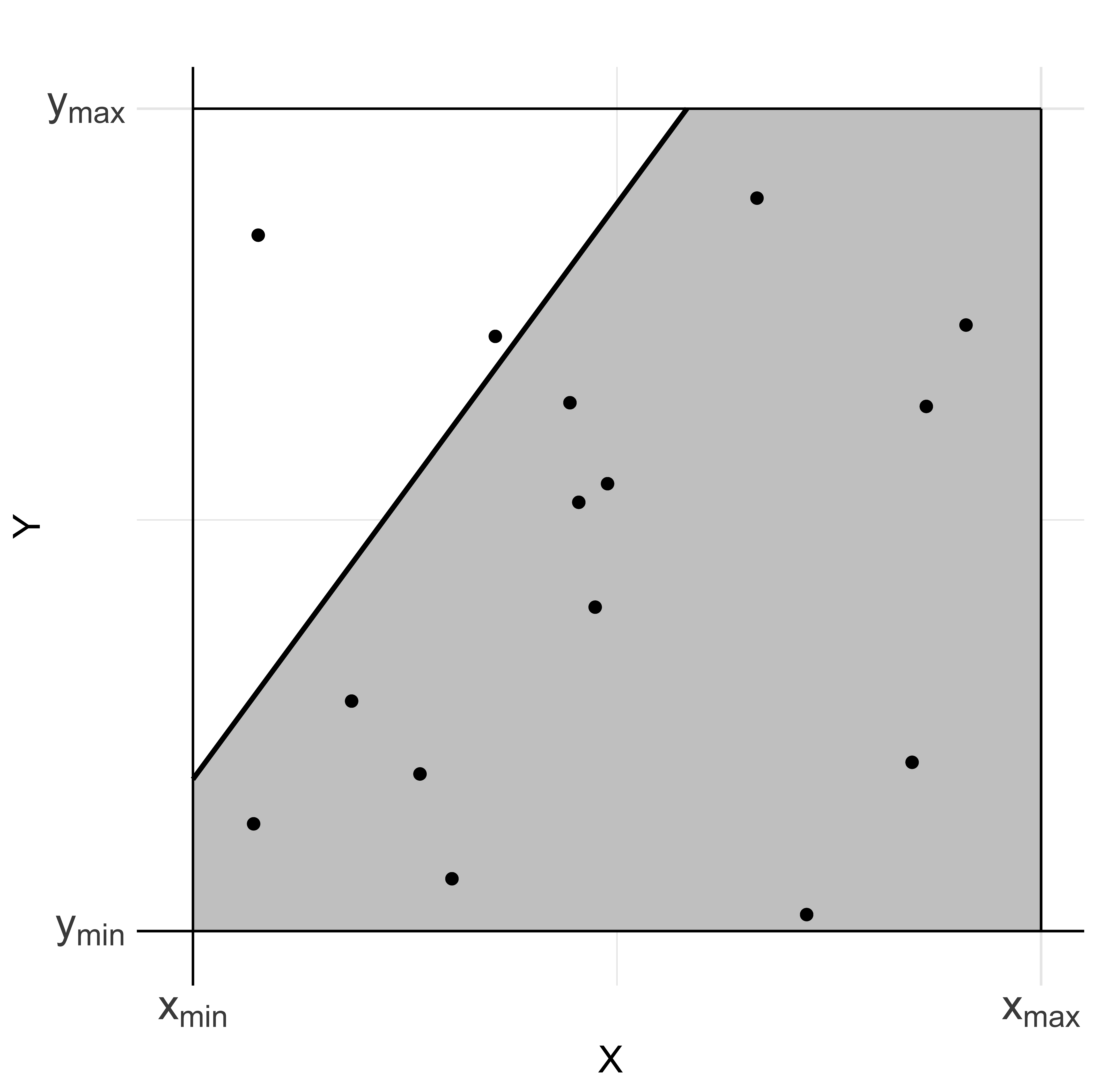
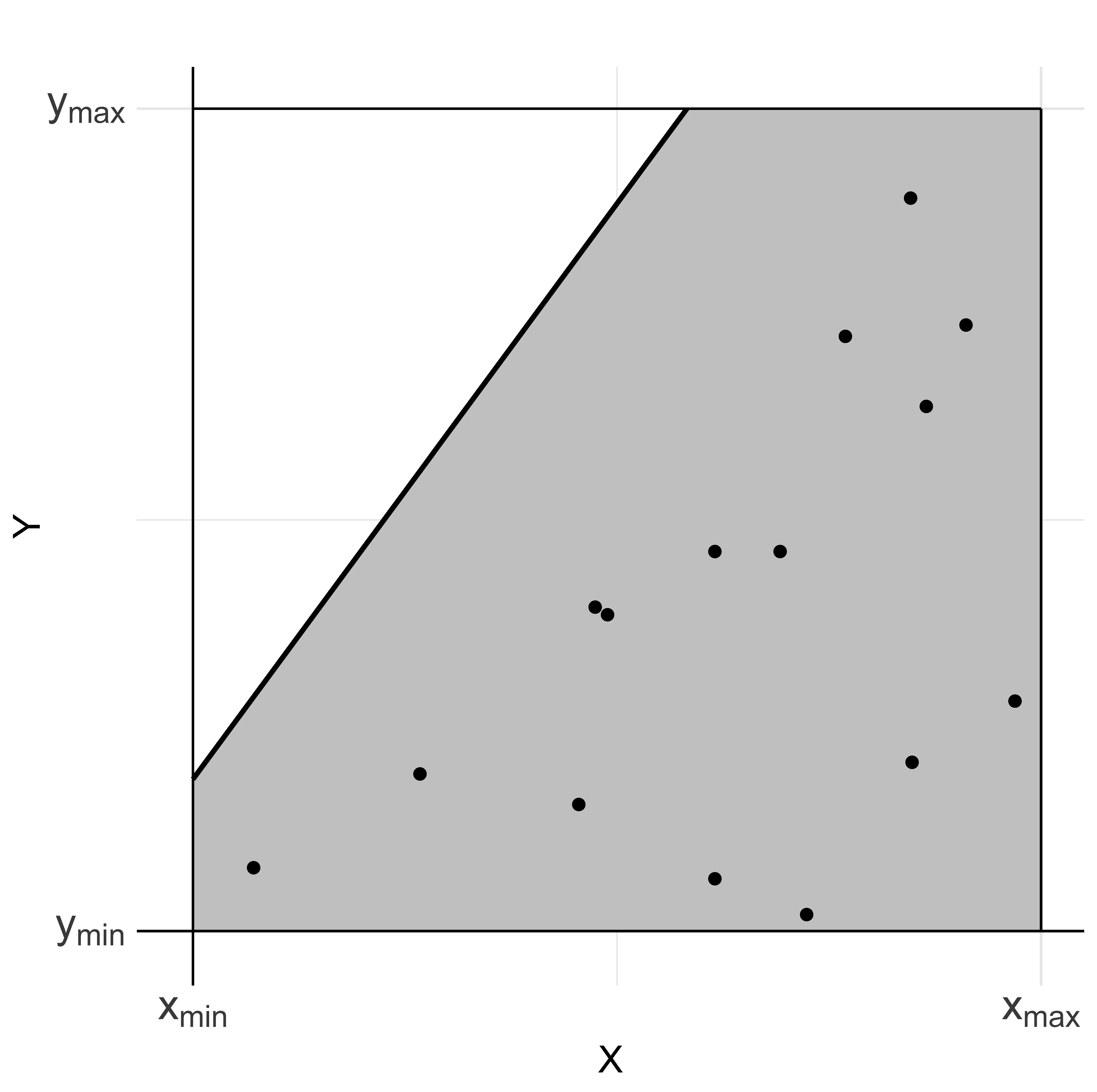
Figure 4.5: Estimation of the ceiling line. Left: points in the ceiling zone. Right: no points in the ceiling zone.

For good model fit nearly all points are in the feasible area. Ceiling accuracy is the percentage of points in the feasible area (on or below the ceiling line):

\[\begin{equation} \tag{4.56} ceiling\,accuracy = \left( 1 - \frac{n_{\text{ceiling zone}}}{n}\right) \times 100\% \end{equation}\]

where $n_{ceiling\,zone}$ is the number of points in the ceiling zone, and $n$ is the total number of points.⁴¹

4.5.4 Purity – noise and exceptions

A disadvantage of the model fit metric ceiling accuracy is that it does not account for the distance between the point and the ceiling line. Points in the ceiling zone that are farther from the ceiling line present a greater challenge to necessity than points that are closer. The purity measure of a point captures the proximity of a point to the ceiling line (Figure 4.6).

Purity: capturing the proximity of a point in the ceiling zone to the ceiling line. $P$ = general point in the ceiling zone; $P_e$ = extreme point in the low-purity part of the ceiling zone. $P_p$ = point in the medium-purity part of the ceiling zone. See the text for an explanation of A and B.

Figure 4.6: Purity: capturing the proximity of a point in the ceiling zone to the ceiling line. $P$ = general point in the ceiling zone; $P_e$ = extreme point in the low-purity part of the ceiling zone. $P_p$ = point in the medium-purity part of the ceiling zone. See the text for an explanation of A and B.

Purity is a measure of closeness of a point P in the ceiling zone to the ceiling. Referring to Figure 4.6-left, it is defined as:

\[\begin{equation} \tag{4.57} purity\,(P) = \frac{\text{size of area of F} \,{\cap}\, \text{LR(P)}} {\text{size of area of LR(P)}} \end{equation}\]

where F is the feasible area, and LR(P) is the area at the lower-right side of point P within the bounding box. Referring to the linear ceiling line in Figure 4.6-left, the numerator of Equation (4.57) is A and the denominator A + B. Therefore, the purity of a point P for a linear ceiling line is:

\[\begin{equation} \tag{4.58} purity\,(P) = \frac{A}{A+B} \end{equation}\]

where the dark-gray area A is the intersection between the feasible area and the LR(P) area, and the dotted area B is the intersection between the ceiling zone and the LR(P) area.

The highest purity value of 1 refers to a point on or below the ceiling line (B = 0, point is not in the ceiling zone). A point above the ceiling line has a purity value < 1. A point in the upper-left corner of the ceiling zone is furthest from the ceiling line, and has the lowest purity value, which equals $1 - d$ where $d$ is the effect size.

Figure 4.6-right shows a dotted line representing points with the same purity value, here 0.9. This line is called the iso-purity line. For a linear ceiling line the iso-purity line is part of an ellipse⁴² and for a stepwise linear function with horizontal and vertical parts it consists of a combination of elliptic and linear segments. The iso-purity line and the ceiling line divide the bounding box into three zones. The low-purity zone is the area above the iso-purity line and within the box where the points are far from the ceiling line. Here the purity is low (purity < 0.9 in Figure 4.6-right). The medium-purity zone is the area between the iso-purity line and the ceiling line, where the points are close to the ceiling (0.9 $\leq$ purity < 1 in Figure 4.6-right). The saturated-purity zone consists of the feasible area including the ceiling line where purity = 1.

Two model fit metrics are derived from the purity measure: noise and exceptions.

The metric noise ($ns$) quantifies uncertainty around the ceiling line due to minor deviations. For good model fit there should be only a limited percentage of points in the medium-purity zone.⁴³

The model fit metric exceptions ($ex$) quantifies violations in the ceiling zone far from the ceiling line, indicating how strict (or tolerant) the necessity claim is. With a deterministic perspective on necessity no cases are allowed in the low-purity zone. If a rare point exists in the low-purity zone, this point may be considered an exception if measurement error and sampling error are excluded. For a typicality perspective, rare exceptions may be permitted in this zone. The proposed model fit metric exceptions captures the number of cases in the low-purity zone.⁴⁴

4.5.5 Solidity – support and spread

To ensure high levels of ceiling accuracy and low levels of noise, a high ceiling line well above the points may be selected as illustrated in Figure 4.5-right. However, when the selected ceiling line is far away from points under the ceiling, it may not be informative in the sense that no or only a few points are constrained by the condition, which can make the necessary condition trivial. When more points are close to the ceiling, more points are constrained by the condition and the necessity of the condition becomes more relevant. Solidity is a measure of closeness of a point P in the feasible area to the ceiling as illustrated in Figure 4.7.

Solidity: capturing the proximity of a point in the feasible area to the ceiling line. $P$ = general point in the feasible area. $P_s$ = point in the medium-solidity part of the feasible area. See the text for an explanation of A and B.

Figure 4.7: Solidity: capturing the proximity of a point in the feasible area to the ceiling line. $P$ = general point in the feasible area. $P_s$ = point in the medium-solidity part of the feasible area. See the text for an explanation of A and B.

Referring to Figure 4.7-left, it is defined as:

\[\begin{equation} \tag{4.59} solidity(P) = \frac{\text{size of area of C} \,{\cap}\, \text{UL(P)}} {\text{size of area of UL(P)}} \end{equation}\]

where C is the ceiling zone, and UL(P) is the area at the upper-left side of point P within the bounding box. Referring to the linear ceiling line in Figure 4.7-left, the numerator of Equation (4.59) is A and the denominator A + B. Therefore, the solidity equation for a linear ceiling line is:

\[\begin{equation} \tag{4.60} solidity\,(P) = \frac{A}{A+B} \end{equation}\]

where the dark-gray area A is the intersection between the ceiling zone and the UL(P) area, and the dotted area B is the intersection between the feasible area and the UL(P) area. The highest solidity value of 1 refers to a point on or above the ceiling line (B = 0, point is not in the feasible area). A point below the ceiling line has a solidity value < 1. A point in the lower-right corner of the feasible area is furthest from the ceiling line, and has the lowest solidity value.

Figure 4.7-right shows a dotted line representing points with the same solidity value, here 0.8. For a linear ceiling line the iso-solidity line is part of an ellipse. The iso-solidity line and the ceiling line divide the bounding box into three zones. The low-solidity zone is the area below the iso-solidity line and within the bounding box where the points are far from the ceiling line. Here the solidity is low (< 0.8 in Figure 4.7-right). The medium-solidity zone is the area between the iso-solidity line and the ceiling line, where the points are close to the ceiling. Here the solidity is high, though not perfect (0.8 $\leq$ solidity < 1 in Figure 4.7-right). The saturated-solidity zone consists of the ceiling zone and the ceiling line where the solidity = 1.

Details of the rationale for selecting the specific distance measure for purity and solidity can be found in (Kuik & Dul, 2026).⁴⁵

For good model fit there should be at least a certain percentage of points on the ceiling line or in the medium-solidity zone, which may represent support for necessity. Model fit metric support ($su$) quantifies how strongly the data in the feasible area support the ceiling.⁴⁶

While the model fit metric support evaluates the percentage of points on and just below the ceiling to support the ceiling, those points may be clustered and only support certain parts of the line. Preferably all parts of the ceiling are supported. The model fit metric spread ($sp$) indicates how evenly the $x$-positions of the supporting points cover the range ($x_{\min},x_{\max}$). To compute spread, the number of points on the ceiling line ($satS$) and in the medium-solidity zone ($medS$) are selected, and their $X$-values ($x_i$ for $i=1,\ldots,n$) are obtained. For this set of $n$ points the coefficient of variation ($CV$) is calculated by dividing the standard deviation ($sd$) by the mean ($\bar{x}$) as follows:

\[\begin{equation} \tag{4.61} \bar{x} = \frac{1}{n}\sum_{i=1}^n x_i \end{equation}\]

\[\begin{equation} \tag{4.62} sd = \sqrt{\frac{1}{n-1}\sum_{i=1}^n (x_i - \bar{x})^2} \end{equation}\]

\[\begin{equation} \tag{4.63} CV = \frac{sd}{\bar{x}} \end{equation}\]

To obtain a metric of evenness, the coefficient of variation is transformed as follows:
\[\begin{equation} \tag{4.64} spread = \frac{1}{1 + \frac{sd}{\bar{x}}} \end{equation}\]

The spread metric ranges from 0 to 1. High spread values (e.g., $\ge$ 0.5) are favored over low spread values. Spread is undefined when $\bar{x} = 0$, which can occur when $x$-values are negative or zero; min-max normalization can avoid this.

4.5.6 Sharpness

The ceiling line serves as a clear boundary that distinguishes the ceiling zone from the feasible area. Sharpness ($sh$) refers to the abrupt change in point density when transitioning between the ceiling zone and the feasible area, and vice versa. Sharpness implies that the density of points in the medium-purity zone (medP; the area between the iso-purity line and the ceiling line) excluding the points on the ceiling line, is much lower than the density of points in the medium-solidity zone (medS; the area between the iso-solidity line and the ceiling line) excluding the points on the ceiling line, as illustrated in Figure 4.8.

Point $P_s$ is in the medium-solidity zone of the feasible area between ceiling line and iso-solidity line (dotted). Point $P_p$ is in the medium-purity zone of the ceiling zone between ceiling line and iso-purity line (dotted). Point $P_e$ is in the low-purity (empty) zone of the ceiling zone outside and may be considered an exception.

Figure 4.8: Point $P_s$ is in the medium-solidity zone of the feasible area between ceiling line and iso-solidity line (dotted). Point $P_p$ is in the medium-purity zone of the ceiling zone between ceiling line and iso-purity line (dotted). Point $P_e$ is in the low-purity (empty) zone of the ceiling zone outside and may be considered an exception.

sharpness is defined as:

\[\begin{equation} \tag{4.65} sharpness = \begin{cases} \frac{medS}{medS+medP} & \text{if } medS + medP \neq 0 \\ \text{NA} & \text{otherwise} \\ \end{cases} \end{equation}\]

where medS is the number of points in the medium-solidity zone excluding the points on the ceiling line, medP is the number of points in the medium-purity zone excluding the points on the ceiling line, and NA indicates that a value is not available. Sharpness defines among the cases that lie close to the ceiling (in the ribbon, see below), what fraction are on the “correct” side (below the ceiling) rather than violating it (above the ceiling). Sharpness has a value between 0 and 1. A sharpness value of 0.5 means that there is no distinction in density of points close above and close below the ceiling line. Sharpness above 0.5 indicates that there are more points close below the ceiling line than close above the ceiling line (as intended).

Table 4.1 shows sharpness values for different values of medP and medS.⁴⁷

Table 4.1: Sharpness values for different combinations of points in the medium-purity zone (rows) and medium-solidity zone (columns). Sharpness > 0.8 is shown in bold.
	0.1	0.2	0.3	0.4	0.5	0.6	0.7	0.8	0.9	1
0.1	0.5	0.67	0.75	0.8	0.83	0.86	0.88	0.89	0.9	0.91
0.2		0.5	0.6	0.67	0.71	0.75	0.78	0.8	0.82	0.83
0.3			0.5	0.57	0.62	0.67	0.7	0.73	0.75	0.77
0.4				0.5	0.56	0.6	0.64	0.67	0.69	0.71
0.5					0.5	0.55	0.58	0.62	0.64	0.67
0.6						0.5	0.54	0.57	0.6	0.62
0.7							0.5	0.53	0.56	0.59
0.8								0.5	0.53	0.56
0.9									0.5	0.53
1.0										0.5

4.5.7 NCA ribbon

The NCA ribbon is the combination of the medium-purity zone and the medium-solidity zone. It represents a type of uncertainty area around the ceiling line. It differs from a confidence interval in statistics but serves a similar goal to capture precision. The ribbon is the geometric area calculated from the ceiling line with specified medium-purity and medium-solidity zones (e.g., 0.9-iso and 0.8-iso, respectively), where a specified maximum (purity) or minimum (solidity) number of points (cases, observations) are located. Few points in the medium-purity zone and many points in the medium-solidity zone means high precision; more points in the medium-purity zone and fewer points in the medium-solidity zone means lower precision.

4.5.8 Summary model fit metrics

The eight metrics of NCA’s model fit with example guidelines are summarized in Table 4.2. The model fit metrics are part of the broader concept of credibility. NCA’s credibility for identifying necessary conditions is discussed in Chapter 6.

Table 4.2: Model fit metrics for NCA
Metric	Description	Symbol	Guideline
Complexity	Half of ceiling degrees of freedom.	$cp$	Balance.
Fit	Alignment with boundary pattern (% effect size compared to CE-FDH effect size).	$ft$	High (e.g., $ft$ ≥ 80%).
Ceiling accuracy	Percentage of points in the feasible area.	$ca$	High (e.g., $ca$ ≥ 95%).
Noise	Percentage of points in the ceiling zone near the ceiling (medP-zone).	$ns$	Low (e.g., $ns$ ≤ 5%; 0.9 iso-purity).
Exceptions	Number of points in the ceiling zone far from the ceiling (lowP-zone).	$ex$	Very low (e.g., $ex$ ~0).
Support	Percentage of points in the feasible area on or near the ceiling (medS-zone).	$su$	High (e.g., $su$ ≥ 5%; 0.8 iso-solidity).
Spread	Evenness of $x$-positions of points on or near the ceiling (medS-zone).	$sp$	High (e.g., $sp$ ≥ 0.5).
Sharpness	Relative density of points in medium-purity (medP) and medium-solidity (medS) zones.	$sh$	High (e.g., $sh$ > 0.8).

4.6 Multiple necessary conditions

Until now the mathematics of necessity has been evaluated by analyzing a single pair of variables: one condition ($X$) and one outcome ($Y$). $X$ and $Y$ represent two (related) properties of the phenomenon of interest, and the relationship between these two properties is analyzed using geometry and algebra in the $XY$-plane. This is NCA’s basic approach, which analyzes necessary conditions one by one. This section first formalizes NCA’s basic approach of analyzing single necessary conditions. Subsequently, it illustrates this reasoning with an example and gives the arguments for it. Finally, the section shows how several linked necessary conditions can be analyzed as a chain of necessity.

4.6.1 Formalization of single condition approach

NCA intentionally reduces causal complexity by reducing a multidimensional constraint structure to single-condition necessity relations by projection, and assumes that these overall necessity constraints manifest as observable ceilings in the empirical (natural) distribution.

The formalization is as follows.⁴⁸ Let $Y \in \mathbb{R}$ denote an outcome variable and let
$\mathbf{X} = (X_1, \ldots, X_J)$ denote a vector of $J$ conditions. Assume that the data-generating process implies an upper bound on $Y$ given by a (possibly unknown and complex) function:

\[\begin{equation} \tag{4.66} Y \le f(\mathbf{X}) \end{equation}\]

where $\mathbf{X}$ is a vector of conditions and $f$ defines a multidimensional ceiling surface.

NCA does not attempt to model or estimate $f(\mathbf{X})$. Instead, for each condition $X_j$, NCA considers the projection of the feasible set onto the $(X_jY)$-plane:

\[\begin{equation} \tag{4.67} {(x_j, y) : \exists \mathbf{x}_{-j}\ \text{such that}\ y \le f(x_j, \mathbf{x}_{-j})}. \end{equation}\]

This projection induces a bivariate model with a ceiling function:

\[\begin{equation} \tag{4.68} Y \le f_j(X_j), \end{equation}\]

where \[\begin{equation} \tag{4.69} f_j(x_j) = sup_{\mathbf{x}_{-j}} f(x_j, \mathbf{x}_{-j}), \end{equation}\] and $\mathbf{x}_{-j}$ denotes all conditions except $X_j$.

The function $f_j(x_j)$ defines the projected ceiling for condition $X_j$. The function $f(x_j, \mathbf{x}_{-j})$ represents the multidimensional ceiling, that is, the maximum attainable value of $Y$ for a given combination of all conditions. For a fixed value $x_j$, the supremum operator $\sup_{\mathbf{x}_{-j}}$ takes the least upper bound of the ceiling $f(x_j, \mathbf{x}_{-j})$ across all admissible values of the remaining conditions. Thus, $f_j(x_j)$ is the highest outcome level that can be achieved at condition level $x_j$ under the most permissive setting of the other conditions. Thus, even if all other conditions take their most lenient possible values, the outcome $Y$ cannot exceed the ceiling value $f_j(x_j)$.

In the context of necessity analysis, this construction ensures that the ceiling function $f_j$ captures the overall necessity constraint imposed by $X_j$: regardless of how the other conditions are configured, the outcome $Y$ cannot exceed $f_j(x_j)$. The empty space above the ceiling is NCA’s key interest, not the feasible area below the ceiling. Assuming a well-covered sample, meaning that for each $x_j$ the data include sufficiently permissive realizations of the unobserved conditions so that the upper boundary is observed, the estimated ceiling line is not biased by third variables that are omitted from the analysis. Conversely, insufficient boundary coverage (e.g., due to limited sampling or selection that removes near-boundary cases) may lead to underestimation of the ceiling (the true ceiling is higher) and thus overestimation of the effect size (the true effect size is smaller).

In other words, NCA assumes that the projected ceiling $f_j$ is recoverable from the empirical joint distribution of ($X_j,Y$), generated under real-world conditions (the natural distribution) and incorporating all interactions, dependencies, and selection mechanisms among the conditions. Under this coverage assumption, the observed data exhibit an empty region above $f_j(X_j)$, making the estimated ceiling a candidate for causal interpretation with additional theory.

4.6.2 Illustration

Section 3.3 discusses a necessity theory with multiple necessary conditions (Figure 3.2). For example, Figure 3.2-left shows a theory that includes three properties of the phenomena (three conditions). In mathematical terms, each condition is a dimension of the multi-dimensional space that models the phenomena. Thus, a model with two conditions $X_1$ and $X_2$, and one outcome $Y$ results in a three-dimensional space. The $XY$-plot becomes a three-dimensional $X_1X_2Y$-space.

NCA’s overall (projected) necessity property is illustrated in Figure 4.9, which shows a volcano mountain where $X_1$ is the horizontal location in one direction, $X_2$ the horizontal location in another direction, and $Y$ the vertical elevation.⁴⁹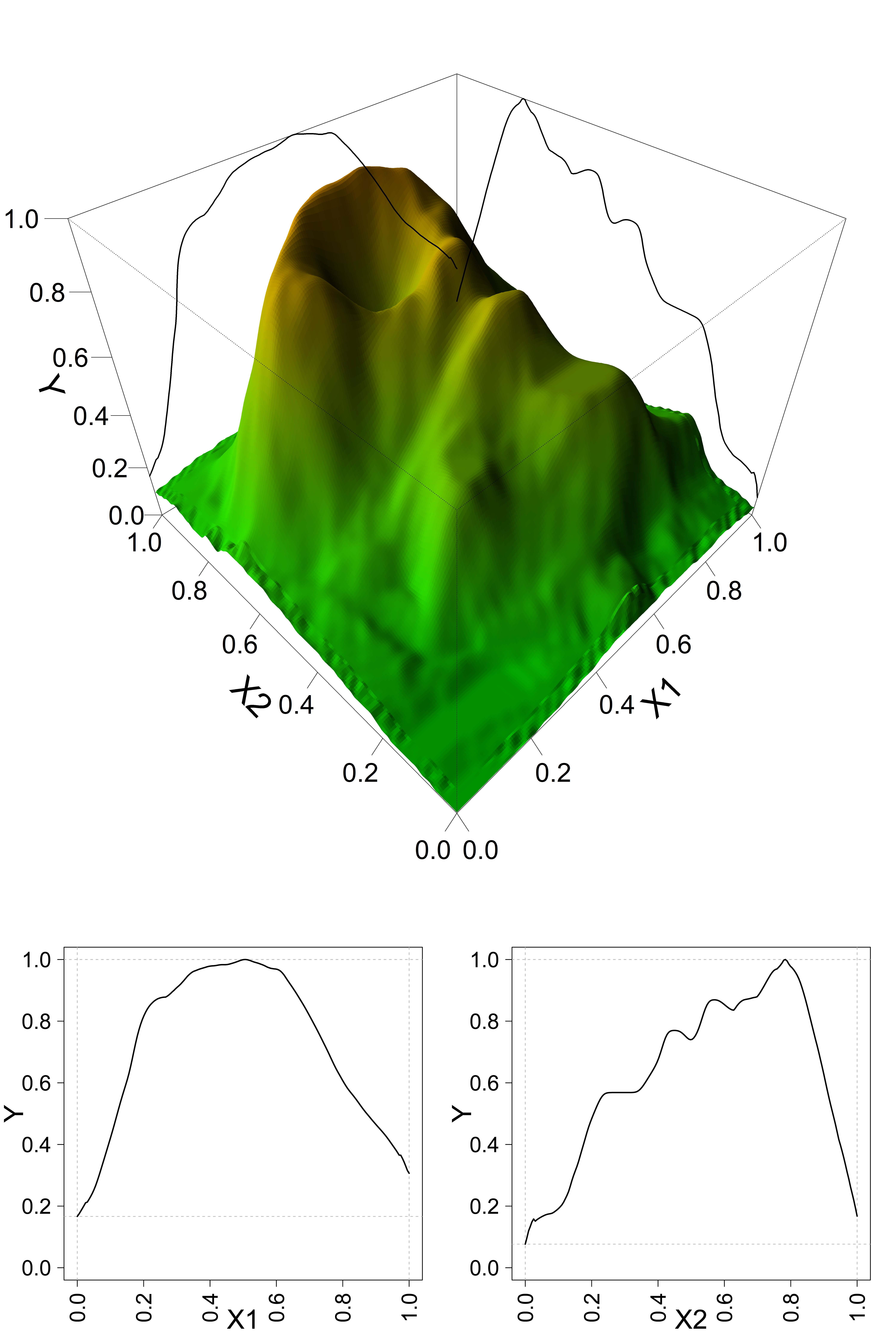

Figure 4.9: A nonlinear three-dimensional ceiling (surface) and its projections on the $X_1Y$ and $X_2Y$-planes (non-linear ceiling lines).

For example, a point within the mountain can be identified by specific values of $X_1$, $X_2$ and $Y$. The height of the mountain is a ceiling surface, which is the set of points representing different mountain heights depending on specific values of $X_1$, $X_2$. The ceiling surface is a very complex function. NCA is not interested in modeling or estimating the multidimensional ceiling (maximum value of the outcome for given combinations of values of the conditions). In contrast, NCA takes the projection of a multidimensional ceiling onto each $X_jY$-plane, resulting in separate ceiling lines for each condition. This projected overall ceiling line in an $X_jY$-plane represents the global necessity of the single condition $X_j$ for outcome $Y$ and is interpreted independently of other conditions and the rest of the causal structure. It is assumed that this global necessity (overall ceiling line) manifests in the real world and can be observed in the empirical (natural) distribution.

The projections of the three-dimensional ceiling surface of the volcano mountain on the $XY$-planes result in non-linear ceiling lines (Figure 4.9). When the three-dimensional ceiling surface is linear (e.g., $Y = (X_1 + X_2)/2$), the projections result in linear ceiling lines, as shown in Figure 4.10.

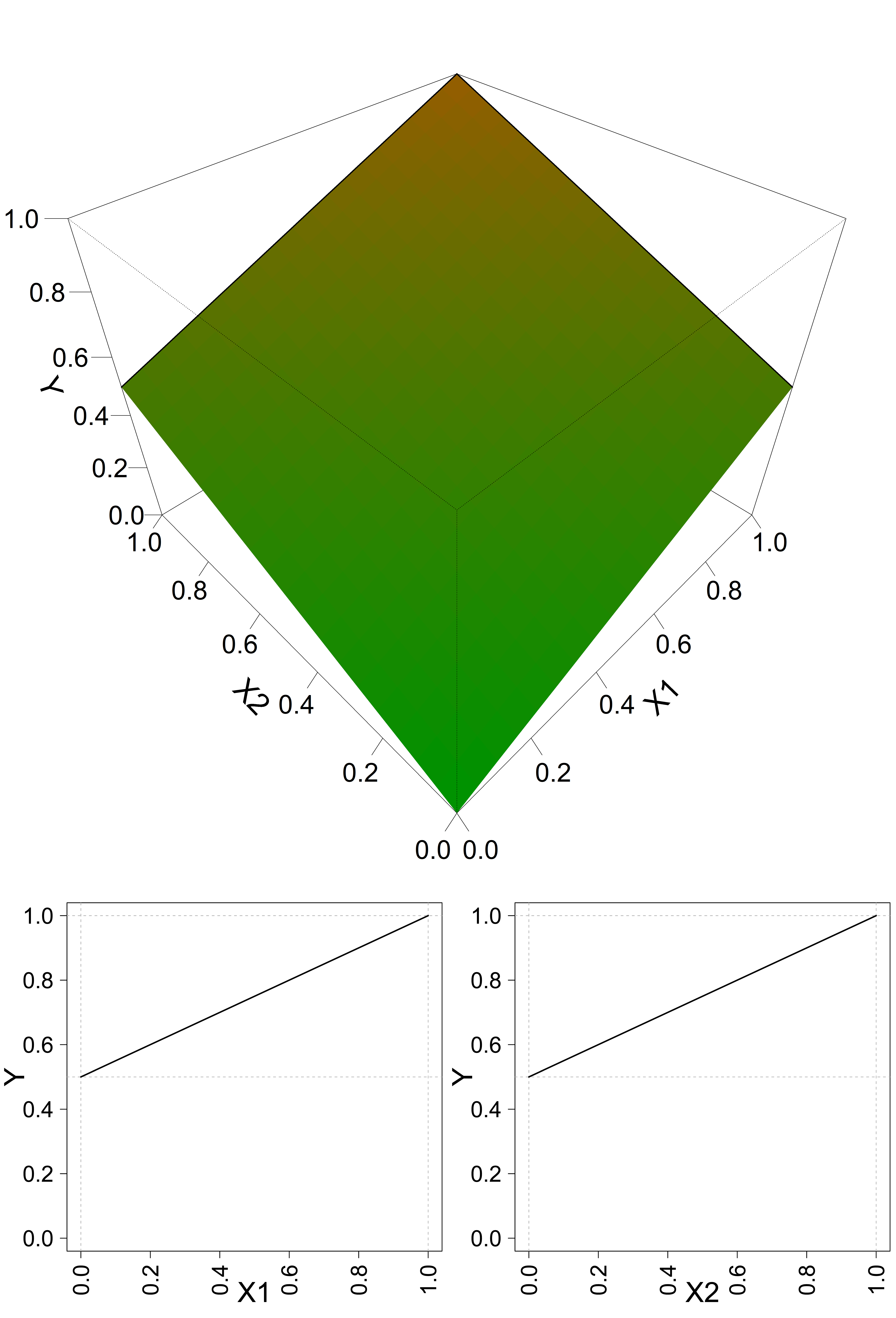
Figure 4.10: A linear multivariate three-dimensional ceiling $Y = (X_1 + X_2)/2$ and its projections on the $X_1Y$- and $X_2Y$-planes (linear ceiling lines).

In a multidimensional space, NCA considers one projection at a time and therefore one condition at a time. With several conditions, NCA conducts successive analyses by considering the ceilings in the separate $X_jY$-planes. For example, with two conditions ($X_1$ and $X_2$), two separate analyses are performed: one in the $X_1Y$-plane and one in the $X_2Y$-plane. In geometric terms, NCA places a ceiling surface over the data and takes its orthogonal projections onto the $X_1Y$- and $X_2Y$-planes. Each condition thus has its own ceiling line, $f_1(X_1)$ and $f_2(X_2)$. Consequently, for a given value $Y = y_c$ two conditions must be satisfied: $X_1 \geq x_{1c}$ AND $X_2 \geq x_{2c}$. Therefore, the maximum possible $Y = y_c$ for given values $X_1 = x_{1c}$, and $X_2= x_{2c}$ is

\[\begin{equation} \tag{4.70} y_c = min \{f_1(x_{1c}), f_2(x_{2c})\} \end{equation}\]

where $y_c$ is a particular outcome value, $x_{jc}$ is the necessary value of the $j$-th condition, and $f_j$ is the ceiling line of condition $X_j$.

With more than two conditions, there is a multidimensional ceiling with projections $f_j(X_j)$.

The mathematical description of a necessity AND-combination of multiple necessary conditions is as follows: for achieving an outcome level $Y = y_c$, all conditions must satisfy $X_j \geq x_{jc}$. The maximum possible value of the outcome $Y = y_c$ for given values $X_j = x_{jc}$ is

\[\begin{equation} \tag{4.71} y_c = min_{j=1,\ldots,J} \{ f_j(x_{jc}) \} \end{equation}\]

Here, $y_c$ is a particular outcome value, $x_{jc}$ is the necessary value of the $j$-th condition, and $f_j$ is the ceiling line associated with condition $X_j$.

Although NCA performs separate analyses for each condition, these analyses are combined and considered jointly in NCA’s bottleneck table (Section 9.11). This allows answering questions such as: “What levels $x_{jc}$ of $X_j$ are necessary for a particular level $Y = y_c$?” and “For given levels $x_{jc}$ of $X_j$, what is the maximum possible level $y_c$ of $Y$?”

4.6.3 Arguments for single condition analyses

There are several reasons why NCA analyzes projections of the multidimensional ceiling.

The first reason is the fundamental choice to focus on single factors that are necessary for an outcome. This distinguishes NCA from conventional analyses that study multi-causal phenomena by considering combinations of factors and their joint effects. A multivariate analysis is the realistic option for predicting the presence of an outcome, because often only a combination of factors (and not a single factor) can produce the outcome. In the case of necessity, however, it is realistic and often theoretically sound to propose that a single factor (a necessary condition as a bottleneck) can prevent the outcome from occurring. Therefore, it is possible and useful to study the necessity of single factors for an outcome using projections.
The second reason is that NCA makes statements about single factors that are necessary independently of other factors in the natural distribution. Thus, the global necessity (with an overall ceiling line) of a single factor does not depend on the level of other factors.⁵⁰ This allows for a “pure” and straightforward interpretation of necessity: “the factor is necessary” rather than “the factor is necessary depending on other factors.” Such pure necessity statements hold independently of other factors. However, the context in which a necessity statement holds is usually not unlimited. The domain in which the necessary condition is assumed to apply must be defined as the theoretical domain of the necessity theory (Chapter 3). Such a specification of the theoretical domain must be part of any necessity theory and related formal hypotheses (Chapter 7).
A third reason is that NCA aims to contribute to parsimonious (simple) theories by avoiding complexity that makes theories difficult to understand and less useful. This is a general goal of theory building in applied sciences. NCA provides an elegant way of reducing complexity, particularly in situations where it is hard or impossible to predict the outcome (e.g., when the explained variances of regression models are low or when accurate prediction require very complex models).
The fourth reason is that practical recommendations derived from single necessary conditions are immediately clear and useful: to achieve a target outcome, all necessary conditions must be satisfied; otherwise, failure of this outcome is guaranteed. The absence of a necessary condition cannot be compensated by other factors, including other necessary conditions.
The final reason is that identifying single necessary conditions is more efficient when using multiple analyses of planes (i.e., several ceiling lines) than when conducting a single analysis of a multidimensional space (i.e., one multidimensional ceiling) followed by projection. Modeling and describing a multidimensional ceiling can be complex (e.g., Figure 4.9). Such a modeling corresponds to frontier analysis (Section 4.4), which aims to predict the maximum outcome for a given combination of factors. In contrast, NCA describes the maximum possible outcome for a single condition and can therefore focus directly on the $XY$-planes and their ceiling lines.

4.6.4 Chain of necessity

Normally, a necessary condition is hypothesized (Chapter 7) and analyzed (Chapter 9) as a necessity relationship between $X$ and $Y$. When multiple necessary conditions are proposed, several overall necessity relationships between $X_j$ and $Y$ may be hypothesized. In addition to such parallel necessary conditions, a serial system, a chain of necessity conditions, can also be hypothesized. In that case, an overall relationship $X_1 \rightarrow Y$ (if present) still holds, but it may be (partly) explained by an indirect chain $X_1 \rightarrow \cdots \rightarrow Y$.

Section 3.3 discussed, in general terms, a necessity theory consisting of a chain of necessary conditions (Figure 3.3). For example, a certain amount of study time may be necessary for a certain level of knowledge retention (quiz score), which in turn may be necessary for a high exam grade. This section analyzes such a chain algebraically. Numerical examples are provided for a chain with two links.

4.6.4.1 Analysis of chain necessity

A general necessity chain consists of a sequence of necessary conditions: the first condition $X_1$, intermediate conditions $X_2, X_3, \ldots, X_J$, and the outcome $Y$:

\[\begin{equation} \tag{4.73} X_1 \rightarrow X_2 \rightarrow X_3 \rightarrow \cdots \rightarrow X_J \rightarrow Y \end{equation}\]

Here, $J$ is the number of necessary conditions (and thus the chain has $J$ links ending in $Y$). For example, an additional intermediate necessary condition between study hours and quiz score could be active class participation (engagement, asking questions).

For each link, a ceiling function bounds the subsequent variable:

\[\begin{equation} \tag{4.74} X_{j+1} \le f_j(X_j), \quad j = 1,\ldots,J-1, \qquad Y \le f_J(X_J). \end{equation}\]

The chain ceiling $f_{\mathrm{chain}}(X_1)$ expresses the implied necessity of $X_1$ for $Y$ through the chain. It is defined as the composition of the link-specific ceiling functions:

\[\begin{equation} \tag{4.75} Y \le f_J\!\big(f_{J-1}(\cdots f_1(X_1)\cdots)\big) = f_{\mathrm{chain}}(X_1). \end{equation}\]

Here, $f_J(X_J)$ is the ceiling function of the last link.

The phrase “a chain is as strong as its weakest link” also applies to a necessity chain. If any link fails to represent a necessity relationship, the chain collapses, and $X_1$ is not necessary for $Y$ through the chain. This situation can occur, for example, when a link is sufficient but not necessary, or when a link is described only by an average effect or correlation without necessity.

Throughout, all variables are assumed to be min–max normalized, all ceilings are defined within the same bounding box, and all variables are assumed to be able to reach the extremes of that bounding box.

In the linear case with the unit bounding box $[0,1] \times [0,1]$, each link is described by a truncated linear ceiling:

\[\begin{equation} \tag{4.76} f_j(X_j) = \min(a_j + b_j X_j,\,1), \qquad j=1,\ldots,J. \end{equation}\]

Here, $a_j$ is the intercept and $b_j$ is the slope. Assume that each link represents the standard case of necessity (a ceiling line on or above the diagonal in the unit box), i.e., $0<a_j<1$ and $1<a_j+b_j$.

The resulting chained ceiling is again linear:

\[\begin{equation} \tag{4.77} Y \le f_{\mathrm{chain}}(X_1) = a_{\mathrm{chain}} + b_{\mathrm{chain}}\,X_1. \end{equation}\]

The chain intercept and slope are:

\[\begin{equation} \tag{4.78} a_{\mathrm{chain}} = \sum_{j=1}^{J} \left( a_j \prod_{k=j+1}^{J} b_k \right), \end{equation}\]

\[\begin{equation} \tag{4.79} b_{\mathrm{chain}} = \prod_{j=1}^{J} b_j, \end{equation}\]

with the convention that an empty product equals $1$.

For ceilings on or above the diagonal, $a_{\mathrm{chain}} \ge 1-b_{\mathrm{chain}}$, which implies $d_{\mathrm{chain}} \le \tfrac{1}{2}b_{\mathrm{chain}}$. In the unit square bounding box $[0,1]\times[0,1]$, the effect size of the (linear) chain ceiling $Y \le a_{\mathrm{chain}} + b_{\mathrm{chain}}X_1$ is:

\[\begin{equation} \tag{4.80} d_{\mathrm{chain}} = \begin{cases} \dfrac{(1-a_{\mathrm{chain}})^2}{2\,b_{\mathrm{chain}}}, & \text{if } a_{\mathrm{chain}} < 1,\\[6pt] 0, & \text{otherwise.} \end{cases} \end{equation}\]

As shown in Equation ((4.78)), each intercept $a_j$ is weighted by the product of downstream slopes $b_{j+1},\ldots,b_J$, and the total intercept $a_{\mathrm{chain}}$ accumulates across the chain. As a result, composing multiple necessary conditions can shift the chain ceiling upward relative to a single link with a comparable slope. Consequently, the chain constraint can become less stringent and may even become non-binding. This explains why, even when each link has a positive effect size, the overall chain can yield a null effect of $X_1$ on $Y$ through the chain.

In other words, for ceilings on or above the diagonal within the bounding box, the “weakest link” principle extends to effect size: the chain effect size is less than or equal to the smallest link effect size.

Since ‘a chain is as strong as its weakest link’, the effect size $d_{chain}$ is less than or equal to the effect sizes of all links:

\[\begin{equation} \tag{4.85} d_{\text{chain}} \leq \min(d_1, d_2, \ldots, d_J) \end{equation}\]

where $d_j$ is the effect size of the $j$-th link in the chain.

4.6.4.2 Numeric examples

When the chain consists of two links and assuming ceiling lines above the diagonal, the intercept and slope of the chain necessity function of Equations (4.78) and (4.79), reduce to:

\[\begin{equation} \tag{4.86} a_{\text{chain}} = a_1b_2 + a_2 \end{equation}\]

\[\begin{equation} \tag{4.87} b_{\text{chain}} = b_1b_2 \end{equation}\]

If all variables are min-max normalized to $[0,1]$, the effect size of each link is:

\[\begin{equation} \tag{4.81} d_j = \frac{(1 - a_j)^2}{2b_j} \end{equation}\]

The equation for effect size $d_{chain}$ of the chain necessity of $X_1$ for $Y$ is:

\[\begin{equation} \tag{4.88} d_{\text{chain}} = \begin{cases} \displaystyle \frac{(1 - a_{\text{chain}})^2}{2b_{\text{chain}}}, & \text{if } a_{\text{chain}} < 1 \\ 0, & \text{otherwise} \end{cases} \end{equation}\]

Two numeric examples of a chain consisting of two links (with ceiling lines above the diagonal) illustrate the behavior that the chain is as strong as its weakest link. In the first example, the two ceiling functions are:

\[\begin{align*} f_1(X_1) = 0.4 + 2.0 \cdot X_1 \\ f_2(X_2) = 0.2 + 1.0 \cdot X_2 \end{align*}\]

According to Equations ((4.86)) and ((4.87)) the intercept and slope for the chain ceiling line are:

\[\begin{align*} a_{chain} = 0.6 \\ b_{chain} = 2.0 \end{align*}\]

Following Equation (4.81), the two effect sizes $d_1$ and $d_2$ are:

\[\begin{align*} d_1 = \frac{(1 - 0.4)^2}{2 \cdot 2.0} = \frac{0.36}{4.0} = 0.09 \\ d_2 = \frac{(1 - 0.2)^2}{2 \cdot 1.0} = \frac{0.64}{2.0} = 0.32 \end{align*}\]

According to Equation (4.88) the chain effect size is:

\[\begin{equation} \tag{4.42} d_{chain} = \frac{(1 - 0.6)^2}{2 \cdot 2.0} = \frac{0.16}{4} = 0.04 \end{equation}\]

The three $XY$-plots are shown in Figure 4.11.

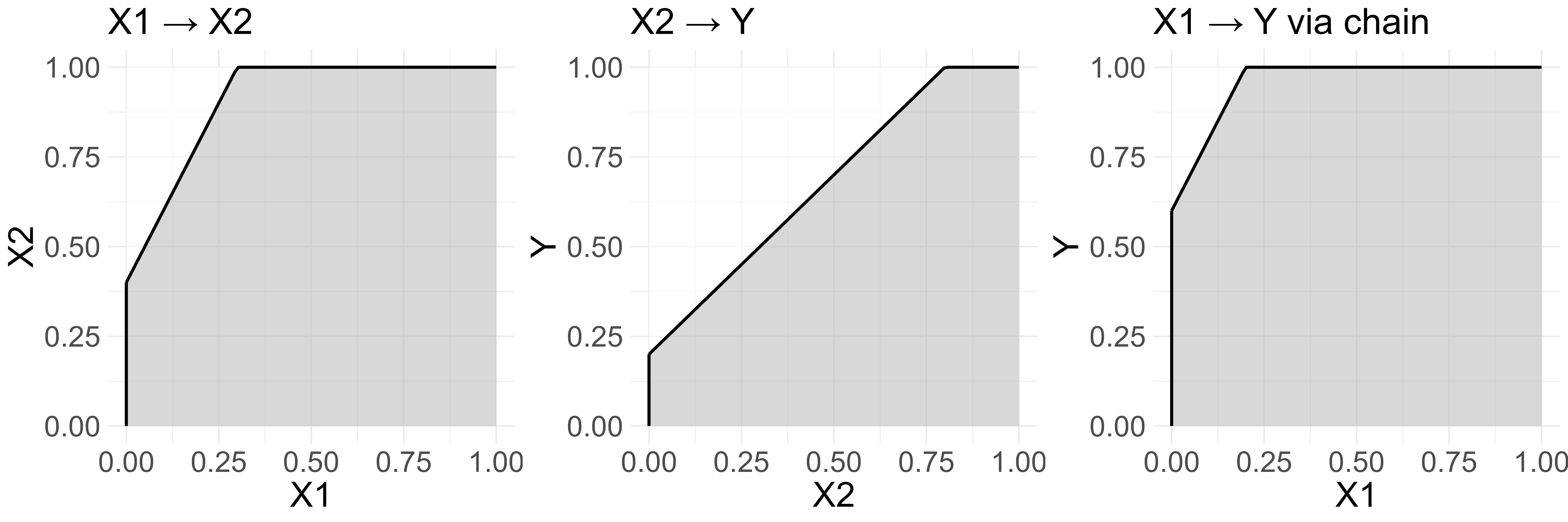
$Example of a necessity chain. The effect sizes of the links are: $X_1 \rightarrow X_2$ = 0.09, $X_2 \rightarrow Y$ = 0.32, $X_1 \rightarrow Y$ = 0.04.$

Figure 4.11: Example of a necessity chain. The effect sizes of the links are: $X_1 \rightarrow X_2$ = 0.09, $X_2 \rightarrow Y$ = 0.32, $X_1 \rightarrow Y$ = 0.04.

The second example is an example where chain necessity vanishes. Two ceiling functions are: \[\begin{align*} f_1(X_1) = 0.4 + 0.7 \cdot X_1 \\ f_2(X_2) = 0.7 + 0.8 \cdot X_2 \end{align*}\]

According to Equations ((4.86)) and ((4.87)), the intercept and slope for the composite ceiling lines are: \[\begin{align*} a_{chain} = 1.02 \\ b_{chain} = 0.56 \end{align*}\]

According to Equation (4.81), the two effect sizes $d_1$ and $d_2$ are: \[\begin{align*} d_1 = \frac{(1 - 0.4)^2}{2 \cdot 0.7} = \frac{0.36}{1.4} \approx 0.26 \\ d_2 = \frac{(1 - 0.7)^2}{2 \cdot 0.8} = \frac{0.09}{1.6} \approx 0.06 \end{align*}\]

Referring to Equation (4.88), the chain effect size is: \[\begin{equation} \tag{4.89} d_{chain} = 0 \end{equation}\]

The three $XY$-plots are shown in Figure 4.12.

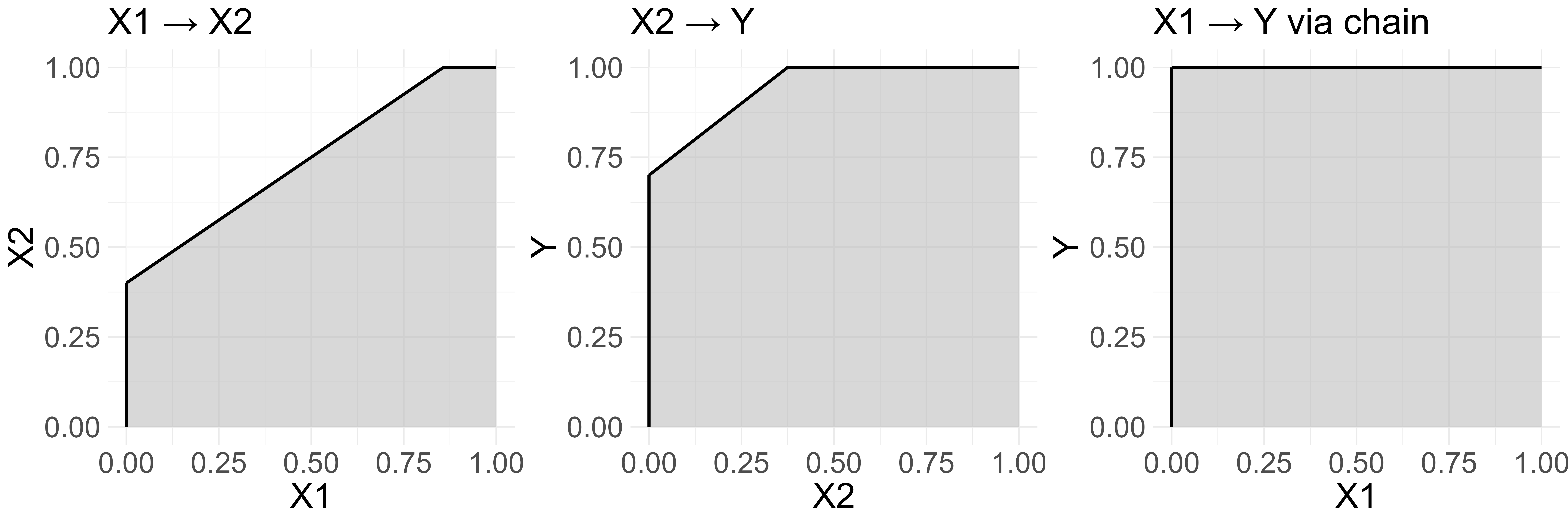
$Example of a necessity chain. The effect sizes of the links are: $X_1 \rightarrow X_2$ = 0.26, $X_2 \rightarrow Y$ = 0.06, $X_1 \rightarrow Y$ = 0.$

Figure 4.12: Example of a necessity chain. The effect sizes of the links are: $X_1 \rightarrow X_2$ = 0.26, $X_2 \rightarrow Y$ = 0.06, $X_1 \rightarrow Y$ = 0.

The examples illustrate that the chain effect size is smaller than the link effect sizes, and that the chain effect size can be zero while those of the links are not.

References

Chen, P.-K. A. (2026). Entrepreneurial resilience learning in higher education: The role of metaverse-constructed ecosystems. The International Journal of Management Education, 24, 101300. https://doi.org/10.1016/j.ijme.2025.101300

Deprins, D., Simar, L., & Tulkens, H. (1984). Measuring labor-efficiency in post offices. In M. Marchand, P. Pestieau, & H. Tulkens (Eds.), The performance of public enterprises: Concepts and measurement (pp. 243–267). North-Holland. https://link.springer.com/chapter/10.1007/978-0-387-25534-7_16

Dul, J. (2016b). Necessary Condition Analysis (NCA): Logic and methodology of “necessary but not sufficient” causality. Organizational Research Methods, 19(1), 10–52. https://doi.org/10.1177/1094428115584005

Dul, J., Hak, T., Goertz, G., & Voss, C. (2010). Necessary condition hypotheses in operations management. International Journal of Operations & Production Management, 30(11), 1170–1190. https://doi.org/10.1108/01443571011087378

Goertz, G., Hak, T., & Dul, J. (2013). Ceilings and floors: Where are there no observations? Sociological Methods & Research, 42(1), 3–40. https://doi.org/10.1177/0049124112460375

Kuik, R., & Dul, J. (2026). Meet the NCA band: Fitting NCA with a ribbon around the necessity ceiling. Rotterdam School of Management, Erasmus University.

Ragin, C. C. (1987). The comparative method: Moving beyond qualitative and quantitative strategies. JSTOR. https://www.jstor.org/stable/10.1525/j.ctt1pnx57?turn_away=true

Also, NCA’s null hypothesis tests for estimation of the $p$-value do not make assumptions about distributions (non-parametric tests, see Section 5.3). However, when statistical simulations are done with NCA such as in Monte Carlo simulations for conducting NCA’s power analysis, the analyst must assume variable distributions including the shape. Any bounded distribution could be selected, for example uniform or truncated normal (Chapters 5 and 6).↩︎
A theoretical scope may apply, for example, when points are obtained from scales with meaningful minimum and maximum values, such as percentage scales, or Likert scales.↩︎
A proof of the acceptability of an affine transformation including linear transformation is presented in Appendix D.↩︎
Although in mathematics the term line is usually reserved for a straight line and curve for a non-straight one, line is used here in the broader, graphical sense to refer to both. Specific shapes of ceiling lines are distinguished with adjectives, such as linear, stepwise linear, or concave piecewise linear.↩︎
For a low-high hypothesis (the absence/low value of $X$ is necessary for the presence/high value of $Y$) the expected empty corner is the upper-right corner (corner 2), etc.↩︎
When a ceiling line has increasing and decreasing parts as for a parabolic ceiling, multiple analyses can be done for each increasing and decreasing part separately. For the increasing part, the empty area is in the upper-left corner, whereas it is in the upper-right corner for the decreasing part. With a parabola-shaped ceiling, an optimum (rather than just low or high) level of $X$ is necessary for a high level of $Y$ (Section 3.7).↩︎
A hypograph is the set of all points that lie on or below the graph of a function.↩︎
For better visibility, the plot can be produced by the NCA software in R as follows: library(NCA); set.seed(123); data <- nca_random (50, 0.3, 1); model <- nca_analysis(data, "X", "Y", ceilings = c("ce_fdh", "cr_fdh", "c_lp", "ce_vrs", "cr_vrs", "QR")); nca_output(model, summaries = FALSE, pdf = TRUE).↩︎
It is also possible as an option in the NCA software that the analyst selects a custom line using a theoretical intercept and the slope.↩︎
Early NCA work proposed quantile regression and stochastic frontier analysis as statistical ceiling estimators (Dul, 2016b; Goertz et al., 2013). Since these approaches lower the ceiling line when more cases appear below the ceiling they are no longer recommended. Stochastic frontier analysis has not been adopted in practice of NCA and is deprecated in the NCA software. Quantile regression remains available, but is rarely used in NCA (for an exception see, P.-K. A. Chen, 2026).↩︎
A low fit value (e.g., < 80%) suggests that the selected ceiling line does not closely follow the boundary.↩︎
A ceiling line can be selected theoretically or estimated from the data. A theoretically selected ceiling line means that the parameters of the ceiling equation are selected a priori, for example, based on previous studies (e.g., in replication studies). It may be that the ceiling line is too low when applied to a new dataset. This would result in having points in the ceiling zone. An estimated ceiling line means that the parameters of the ceiling equation are estimated from the current data. For example, when the CR-FDH technique (Section 4.4) is used, normally some points will be in the ceiling zone.↩︎
For the dichotomous situation Ragin (1987) suggested at least 80% of points should be in the feasible area for support of necessity. In a prototype version of NCA, Dul et al. (2010) suggested at least 95% should be in the feasible area. A lower ceiling accuracy score than for example 95% classifies several cases as not being compatible with strict necessity, which requires further investigation of these cases or a reconsideration of the selection of the ceiling line.↩︎
The conic segment arises from calculations with areas.↩︎
For example, not more than 5% of points may be tolerable noise for a medium-purity zone corresponding to 0.9 iso-purity (in this zone the points have a purity of 0.9 $\leq$ purity < 1).↩︎
Exceptions should be rare (e.g., ~ 0 in the ceiling zone corresponding to purity < 0.9) to justify a typicality causal perspective. No strict rules exist for what number should be considered as “rare.” What matters is that, unlike noise, an exception-case represents a different causal process not captured by necessity, which may be studied separately.↩︎
Various other distance measures such as horizontal, vertical, or perpendicular distance to the ceiling line could be used as a proximity measure, but each has limitations. When using horizontal or vertical distance of point $P$ to the ceiling, the variation in the other direction is ignored, which is problematic when the ceiling line is non-linear. Perpendicular distance could solve this but this distance measure loses its orthogonality under affine transformations (e.g., normalization) of the scope. To address these issues, a proximity measure based on the area between the point’s horizontal and vertical distances and the ceiling line is used. Assuming that the ceiling line is non-decreasing, this area-based measure has several desirable properties: continuity meaning that it varies smoothly with the point’s location, monotonicity meaning that the value increases as the point moves farther from the ceiling line, and invariance meaning that it remains invariant under affine transformations of the scope.↩︎
For example, at least 5% of points could be considered acceptable support with a medium-solidity zone corresponding to 0.8 iso-solidity (in this zone the points have a solidity of 0.8 $\leq$ solidity $\leq$ 1.).The proposed suggestion for iso-solidity is less strict than that for iso-purity. The reason is that purity < 1 violates strict necessity. However, solidity < 1 does not violate necessity. Solidity < 1 implies that the single necessary condition is only less informative for sufficiency. If solidity = 1 all points are on or above the ceiling, which makes the necessary conditions also sufficient. However, assessing the sufficiency of a single condition is not a goal of NCA, which focuses on single factors being necessary. Low solidity may affect sharpness, see Section 4.5.6.↩︎
For good model fit the sharpness should be for example at least 0.8 such that from all points in the ribbon 80% is on the ‘correct’ side.↩︎
The specification of the bounding box is tacitly assumed for simplification.↩︎
Data are from the Maungawhau volcano in Auckland, New Zealand and were obtained from the package .↩︎
When subsamples are drawn it is possible that the ceiling for the subgroup is lower than the ceiling of the total group, but the ceiling can never be higher. This subgroup ceiling may represent a different necessity theory with a different theoretical domain, see Section 11.3.3 and Chapter 7.↩︎

Metric	Description	Symbol	Guideline
Complexity	Half of ceiling degrees of freedom.	\(cp\)	Balance.
Fit	Alignment with boundary pattern (% effect size compared to CE-FDH effect size).	\(ft\)	High (e.g., \(ft\) ≥ 80%).
Ceiling accuracy	Percentage of points in the feasible area.	\(ca\)	High (e.g., \(ca\) ≥ 95%).
Noise	Percentage of points in the ceiling zone near the ceiling (medP-zone).	\(ns\)	Low (e.g., \(ns\) ≤ 5%; 0.9 iso-purity).
Exceptions	Number of points in the ceiling zone far from the ceiling (lowP-zone).	\(ex\)	Very low (e.g., \(ex\) ~0).
Support	Percentage of points in the feasible area on or near the ceiling (medS-zone).	\(su\)	High (e.g., \(su\) ≥ 5%; 0.8 iso-solidity).
Spread	Evenness of \(x\)-positions of points on or near the ceiling (medS-zone).	\(sp\)	High (e.g., \(sp\) ≥ 0.5).
Sharpness	Relative density of points in medium-purity (medP) and medium-solidity (medS) zones.	\(sh\)	High (e.g., \(sh\) > 0.8).