H Demonstration NCA with PLS-SEM
This section demonstrates the steps for combining NCA with SEM (Section 11.4) using an example. This example has been used in four published studies where NCA is combined with PLS-SEM (Hauff et al., 2024; Richter, Schubring, et al., 2020; Richter, Hauff, Ringle, et al., 2023; Sarstedt et al., 2024). The goal of the demonstration is fourfold:
Show how the combined analysis can be done following the flowchart presented in this book.
Show how the proposed BIPMA plot for prioritizing evidence-based action in practice can be produced and how it differs from IPMA and cIPMA.
Show how robustness checks for NCA can be conducted in the context of SEM.
Show how to conduct a combined NCA-SEM analysis with
R.
This demonstration is a replication of the four above studies by using a different software package than the SmartPLS package. The NCA package for R includes all NCA functions and is free. The SmartPLS software may be more user-friendly for users who are not familiar with R, but it is not free and does not include all NCA functions.
The selected example evaluates an extended version of the Technology Acceptance Model (TAM) (Richter, Schubring, et al., 2020). Figure H.1 shows the model consisting of six variables (rectangles) and 9 relationships (arrows).
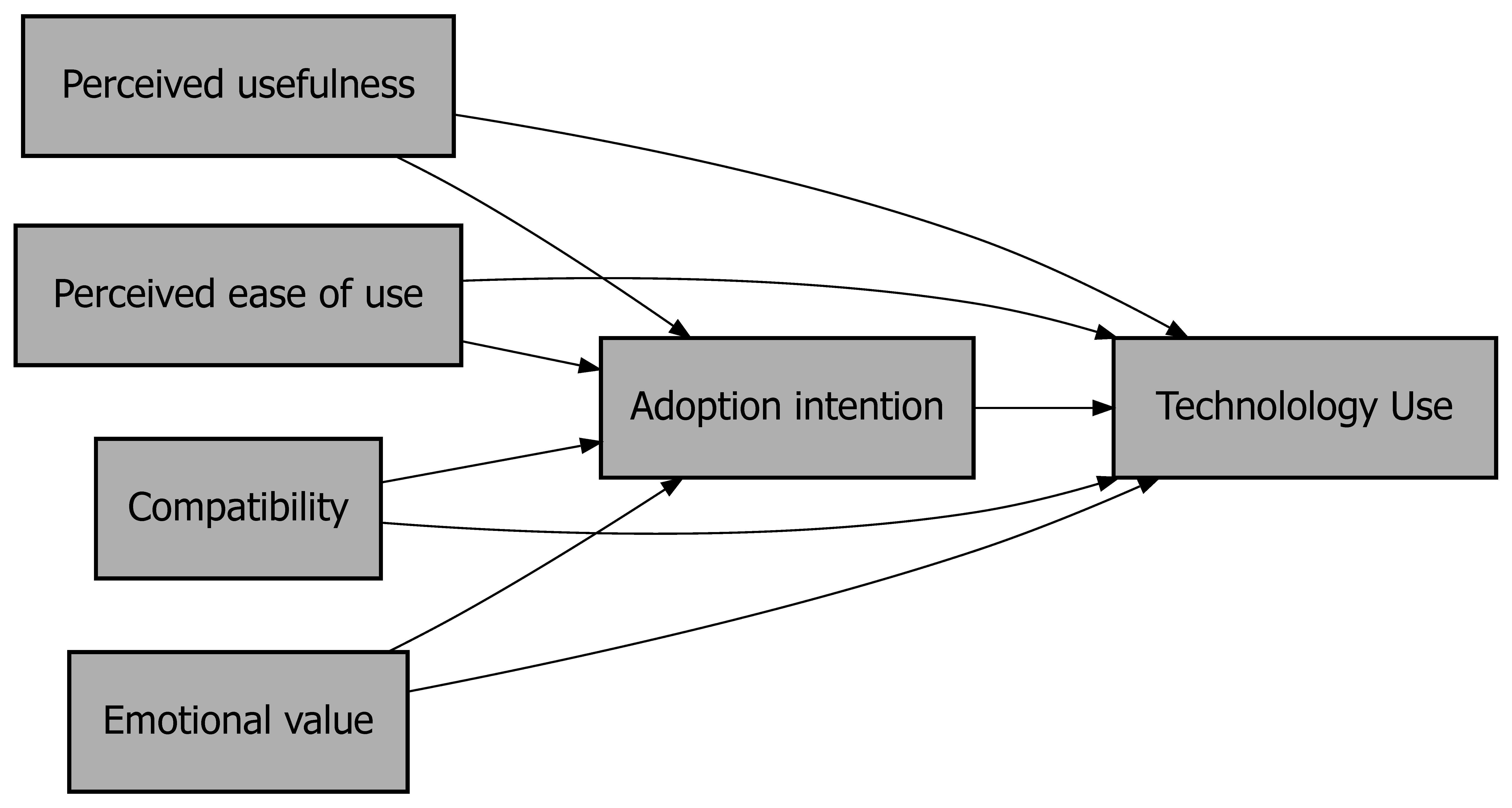
Figure H.1: The extended Technology Acceptance Model (TAM) according to Richter, Schubring, et al. (2020).
For the demonstration, the flowchart of Figure 11.4 is followed. The R packages SEMinR for conducting PLS-SEM, NCA for conducting NCA, and the general purpose R packages ggplot2 and ggrepel for graphics need to be installed. Additional R code for conducting the analysis can be found in Section B.2.
H.1 Step 1: Theorize necessity and probabilistic relationships
It is assumed that the relationships shown in Figure H.1 are theoretically justified from both the perspective of probabilistic sufficiency as well as from the perspective of necessity (Richter, Schubring, et al., 2020). For enhancing the necessity theorizing see Section 7.5.3.
H.2 Step 2: Collect data
The dataset is provided by (Schubring & Richter, 2023) on Mendeley Data, and explained in Richter, Hauff, Kolev, et al. (2023). The dataset needs to be downloaded in the working directory.
The helper function get_indicator_data_TAM imports the dataset, selects relevant columns, and changes the column names for use in SEMinR. The helper function can be downloaded from the book-page: https://jandul.github.io/NCA.
# Get indicator data
source("get_indicator_data_TAM.R")
df <- get_indicator_data_TAM()
head(df, 3)
## PU1 PU2 PU3 CO1 CO2 CO3 EOU1 EOU2 EOU3 EMV1 EMV2 EMV3 AD1 AD2 AD3 USE
## 1 4 3 3 3 3 3 5 5 4 4 3 3 2 2 2 2
## 2 3 1 4 3 3 4 4 4 2 4 4 3 5 4 4 3
## 3 4 4 4 3 3 4 4 4 4 4 4 4 4 4 4 3The original data consists of 174 rows (cases = individuals using e-readers) and 20 columns. The first 16 columns represent the raw indicators of the 6 variables of the TAM model. The last four columns are not considered in this demonstration and are removed from the dataset. After running the helper function, the resulting dataset df is used as input for the PLS-SEM model. The raw indicator scores are measured with 5-point Likert scales, except for the score for Technology use, which is measured with a 7-point Likert scale. The variable names are PU = Perceived usefulness, CO = Compatibility, EOU = Perceived ease of use, EMV = Emotional value, AD = Adoption intention, and USE = Technology use.
H.3 Step 3: Conduct SEM
Following the four original studies, the PLS-SEM approach is selected to estimate the SEM model using the SEMinR package. This package standardizes the raw scores and produces latent construct scores (mean = 0, sd = 1), path coefficients and other output. The helper function estimate_sem_model_TAM conducts the PLS-SEM model estimation. This R function can be downloaded from the book-page: https://jandul.github.io/NCA.
The summary of the results shows the standardized path coefficients and some metrics about model fit:
# Estimate SEM model
# install.packages("seminr") # install the package if needed
source("estimate_sem_model_TAM.R")
TAM_pls <- estimate_sem_model_TAM(df)
summary(TAM_pls)
##
## Results from package seminr (2.5.0)
##
## Path Coefficients:
## Adoption intention Technology use
## R^2 0.539 0.420
## AdjR^2 0.528 0.403
## Perceived usefulness 0.227 0.050
## Compatibility 0.045 0.107
## Perceived ease of use 0.088 0.010
## Emotional value 0.515 0.137
## Adoption intention . 0.437
##
## Reliability:
## alpha rhoA rhoC AVE
## Perceived usefulness 0.723 0.753 0.842 0.642
## Compatibility 0.858 0.859 0.914 0.779
## Perceived ease of use 0.783 0.783 0.873 0.697
## Emotional value 0.914 0.917 0.946 0.853
## Adoption intention 0.938 0.939 0.960 0.889
## Technology use 1.000 1.000 1.000 1.000
##
## Alpha, rhoA, and rhoC should exceed 0.7 while AVE should exceed 0.5The results correspond to those reported in the four original publications using the SmartPLS software.
In addition, the 95% confidence interval of the path coefficients can be obtained using bootstrapping. A path is significant if its 95% bootstrap confidence interval does not include zero. The helper function get_significance_sem.R can be used to find significant direct effects, indirect effects, and total effects as follows. This R function can be downloaded from the book-page: https://jandul.github.io/NCA.
# Estimate significance SEM effects
source("get_significance_sem.R")

# Limit computation time
nboot <- 5000 # set lower for less computation time;
              # for final analysis select 5000
set.seed(123) # for reproducible results
TAM_sig <- get_significance_sem (sem = TAM_pls,
                                 nboot = nboot)
print(TAM_sig)
## Path Direct Indirect Total
## 8 Perceived usefulness -> Adoption intention 0.227 0.000 0.227
## 9 Perceived usefulness -> Technology use 0.050 0.099 0.149
## 2 Compatibility -> Adoption intention 0.045 0.000 0.045
## 3 Compatibility -> Technology use 0.107 0.020 0.127
## 6 Perceived ease of use -> Adoption intention 0.088 0.000 0.088
## 7 Perceived ease of use -> Technology use 0.010 0.038 0.049
## 4 Emotional value -> Adoption intention 0.515 0.000 0.515
## 5 Emotional value -> Technology use 0.137 0.225 0.362
## 1 Adoption intention -> Technology use 0.437 0.000 0.437
## Sig_Direct Sig_Indirect Sig_Total pval_direct pval_total Predicted
## 8 TRUE FALSE TRUE 0.030 0.030 Adoption intention
## 9 FALSE FALSE FALSE 0.602 0.180 Technology use
## 2 FALSE FALSE FALSE 0.690 0.690 Adoption intention
## 3 FALSE FALSE FALSE 0.383 0.294 Technology use
## 6 FALSE FALSE FALSE 0.268 0.268 Adoption intention
## 7 FALSE FALSE FALSE 0.886 0.501 Technology use
## 4 TRUE FALSE TRUE 0.000 0.000 Adoption intention
## 5 FALSE TRUE TRUE 0.121 0.000 Technology use
## 1 TRUE FALSE TRUE 0.000 0.000 Technology useFor the direct paths, three out of nine path coefficients are significant:
Perceived usefulness \(\rightarrow\) Adoption intention (direct effect: 0.227),
Emotional value \(\rightarrow\) Adoption intention (direct effect: 0.515)
and Adoption intention \(\rightarrow\) Technology use (direct effect: 0.437)
For the indirect paths, one out of four paths is significant:
- Emotional value \(\rightarrow\) Adoption intention \(\rightarrow\) Technology use (indirect effect: 0.225)
From the four combined direct and indirect paths (total effect) only one is significant: Emotional value \(\rightarrow\) Adoption intention \(\rightarrow\) Technology (total effect = 0.362).
These results suggest that for increasing Technology use on average, only Emotional value and Adoption intention are effective. Perceived usefulness, Compatibility and Perceived ease of use are not candidates for intervention based on the SEM results as they do not have a significant total effect on Technology use.
H.4 Step 4: Extract latent variable scores
By default, PLS-SEM model estimation produces standardized latent variable scores, and this is the only option in SEMinR version 2.4.2 that was used for the analysis. However, unstandardized scores are preferred as input for NCA, and normalized unstandardized scores are needed for IPMA, cIPMA and BIPMA. The helper function unstandardize calculates the unstandardized latent variable scores from the standardized latent variable scores using procedures described in (Ringle & Sarstedt, 2016), such that the scale of the latent variable scores matches the scale of the original indicator scores. This R function can be downloaded from the book-page: https://jandul.github.io/NCA.
# Unstandardize data
source("unstandardize.R")
dataset <- unstandardize(TAM_pls)
head(dataset, 3)
## Perceived usefulness Compatibility Perceived ease of use Emotional value
## 1 3.276582 3.000000 4.676176 3.322971
## 2 2.668901 3.336436 3.352351 3.663039
## 3 4.000000 3.336436 4.000000 4.000000
## Adoption intention Technology use
## 1 2.000000 2
## 2 4.329378 3
## 3 4.000000 3data.frame (Mean = colMeans(dataset),
Min = apply(dataset, 2, min),
Max = apply(dataset, 2, max)
)## Mean Min Max
## Perceived usefulness 3.569914 1.000000 5
## Compatibility 3.462276 1.000000 5
## Perceived ease of use 4.025616 1.674851 5
## Emotional value 3.806854 1.000000 5
## Adoption intention 3.881627 1.000000 5
## Technology use 3.982759 1.000000 7The resulting dataset with unstandardized latent variable scores is called dataset. The variables are now interpretable according to the Likert scales that were used to measure its raw indicators. The results show that minimum and maximum latent variable scores correspond to the minimum and maximum values of the Likert scale values. There is one exception: the minimum observed latent variable score for Perceived ease of use is 1.67 whereas the minimum value of the scale is 1. Apparently, none of the 174 cases (individuals) scored a value 1 on all three indicators of this latent variable.
The unstandardized latent variable scores can be min-max normalized to obtain normalized unstandardized latent variable scores. Min-max normalization is essential if the predictor variables do not have the same scale values (e.g., one predictor variable is measured with a 1-5-Likert scale while another predictor variable is measured with a 1-7-Likert scale). If the same scale is used for all predictor variables, it is preferred not to normalize the scales and to keep the unstandardized latent variables scores, such that the results are interpretable according to the Likert scale values.
Data can be normalized using the helper function nca_util_normalize of the NCA package in R. The input arguments for this function are the data and the range (theoretical minimum and maximum) of the scale (the observed minimum or maximum values might be different). The range of the scale (e.g., 0-1 or 0-100). For example, (c)IPMA commonly uses a 0-100 normalization of the unstandardized latent variable scores:
# Min-max normalize data
data <- dataset
scale = c(0, 100) #new percentages scale
library(NCA) # use normalize utility of NCA
min_max <- c(rep(c(1,5), 5), c(1,7)) # min and max values of original scale
dataset1 <-  nca_util_normalize(data = data, scale = scale, min_max = min_max)
head(dataset1, 3)
## Perceived usefulness Compatibility Perceived ease of use Emotional value
## 1 56.91456 50.00000 91.90439 58.07427
## 2 41.72252 58.41091 58.80878 66.57599
## 3 75.00000 58.41091 75.00000 75.00000
## Adoption intention Technology use
## 1 25.00000 16.66667
## 2 83.23446 33.33333
## 3 75.00000 33.33333The resulting dataset with 0-100 normalized unstandardized latent variable scores is called dataset1. The variable scores can be interpreted as percentages of the range of the scale. For example, the midpoint 3 of a non-normalized unstandardized 1-5-Likert scale becomes 50 after 0-100 normalization. Note that for the illustrative example normalization is not essential for conducting IPMA, cIPMA or BIPMA because the five predictor variables have the same scale values (1-5-Likert scales).
Since the results of NCA are insensitive to linear transformations (Appendix D), the results are the same for standardized, unstandardized, normalized or non-normalized scores. Unstandardized (normalized or non-normalized) latent variable scores are the preferred input for NCA because of interpretability. The reason is that, in contrast to SEM where a relationship is described in terms of a change of \(X\) producing a change of \(Y\) (e.g., more \(X\) produces more \(Y\)), NCA describes a relationship in terms of the necessity of a level of \(X\) for a level of \(Y\) (level \(x\) of \(X\) is necessary for level \(y\) of \(Y\)). By using interpretable levels linked to the original (unstandardized) scales, NCA results become more insightful.
H.5 Step 5: Conduct NCA
To estimate the necessity of the 9 relationships in the TAM model, 9 necessity analyses are done to obtain necessity effect sizes and \(p\)-values. These analyses are grouped into two multiple NCA’s: one for the outcome Adoption intention (with four conditions: Perceived usefulness, Compatibility, Perceived ease of use, Emotional value), and one for the outcome Technology use (with five conditions: Perceived usefulness, Compatibility, Perceived ease of use, Emotional value, Adoption intention). The remainder of this demonstration focuses on the outcome Technology use, thus only five necessity relationships are analyzed.
In the original four studies that use the example, the analysts make following choices for the NCA analysis:
Ceiling line = CE-FDH.
Effect size threshold level = 0.10.
\(p\)-value threshold level = 0.05.
Scope: empirical scope.
Outlier removal: none.
Target outcome = 85% (only in Hauff et al., 2024; Sarstedt et al., 2024).
For this demonstration, the same choices for the primary NCA analysis are made (and different choices for the robustness checks).
The original studies use standardized scores (Richter, Schubring, et al., 2020), non-normalized unstandardized scores (Richter, Hauff, Ringle, et al., 2023), or 0-100 normalized unstandardized scores (Hauff et al., 2024; Sarstedt et al., 2024) as input for NCA. For this demonstration, the preferred scores from an NCA perspective are used as input data: unstandardized latent variable scores without normalization (because all indicator scales of the conditions use the same Likert scales). NCA can be conducted as follows with the NCA software in R.
library(NCA)
# Limit computation time
test.rep <- 10000 # set lower for less computation time;
                  # for final analysis select 10000
# Conduct NCA - Technology use
set.seed(123) # for reproducible results
model1.technology <- nca_analysis(dataset, 1:5, 6,
                                  ceilings = "ce_fdh",
                                  test.rep = test.rep)
print(model1.technology)
##
## ---------------------------------------------------------------------------## Effect size(s):## ce_fdh p
## Perceived usefulness 0.24 0.001
## Compatibility 0.21 0.000
## Perceived ease of use 0.24 0.016
## Emotional value 0.33 0.000
## Adoption intention 0.29 0.000
## ---------------------------------------------------------------------------# Conduct NCA - Adoption intention
set.seed(123) # for reproducible results
model1.adoption <- nca_analysis(dataset, 1:4, 5,
ceilings = "ce_fdh",
test.rep = test.rep)
print(model1.adoption)##
## ---------------------------------------------------------------------------## ce_fdh p
## Perceived usefulness 0.12 0.003
## Compatibility 0.08 0.009
## Perceived ease of use 0.15 0.008
## Emotional value 0.21 0.000
## ---------------------------------------------------------------------------The results show NCA’s effect size and \(p\)-value of the five conditions for Technology use. The results correspond to those reported in the four original studies using the SmartPLS software. It can be concluded that the five conditions are necessary conditions for Technology use because the three criteria for identifying necessity-in-kind are met:
A necessity hypothesis is formulated and theoretically justified (for the purpose of this demonstration this requirement is assumed to be met).
The effect size is relatively large (\(d \geq\) 0.10).
The \(p\)-value is relatively small (\(p\) < 0.05).
This means that the analysis can continue with an analysis of necessity-in-degree with a bottleneck table that includes all five necessary conditions. This analysis gives information about the minimum level of a condition that is necessary for the target level of the outcome. It also informs if in individual cases a selected target outcome level is achievable, given the observed levels of the conditions. If a case has a value of any condition below the minimum required level for that condition, this case is a ‘bottleneck case’ for that condition. If the case has a condition value above the minimum required level, the case is not a bottleneck case for the condition, but could be a bottleneck case for another conditions. Only when all condition values exceed their respective threshold levels, the case is not a bottleneck case, making the target outcome level achievable.
The use of non-normalized unstandardized latent variable scores and of ‘actual values’ in the bottleneck table ensures a direct link between the values in the bottleneck table and the values of the Likert scales that were used to measure the indicator scores. This means that in NCA’s nca_analysis function, the values of conditions in the bottleneck table must be specified as ‘actual’ using the argument bottleneck.x = 'actual'. Since the outcome variable Technology use has 7 distinct levels, the steps in the bottleneck table preferably correspond to these levels of the outcome. This can be done with the argument steps.
# Bottleneck table Technology use: actual-actual
library(NCA)
bottleneck.y = "actual"
bottleneck.x = "actual"
steps = c(1,2,3,4,5,6,7)
model2.technology <- nca_analysis(dataset,# unstandardized (non-normalized)
                                  1:5, # five conditions
                                  6, # outcome
                                  ceilings = "ce_fdh",
                                  bottleneck.x = bottleneck.x,
                                  bottleneck.y = bottleneck.y,
                                  steps = steps)
nca_output (model2.technology, summaries = FALSE, plots = FALSE,
            bottlenecks = TRUE)
##
## ---------------------------------------------------------------------------## ---------------------------------------------------------------------------
## Y 1 2 3 4 5
## 1 NN NN NN NN NN
## 2 NN NN 2.015 NN NN
## 3 NN NN 2.015 NN NN
## 4 1.628 2.021 2.339 2.986 2.353
## 5 1.628 2.348 2.339 2.986 2.353
## 6 2.925 2.348 2.355 2.986 2.353
## 7 3.648 2.348 3.676 2.986 4.000The outcome variable Technology use is the perceived frequency of utilizing an e-book. The 7 anchor points are 1 = never, 2 = seldom; 3 = several times a month; 4 = once a week; 5 = several times a week; 6 = daily; 7 = several times daily. The condition variables are measured on a 5 point disagree-agree Likert scale where the anchor points range from 1 = strongly disagree to 5 = agree fully. In the original studies (and here) it is assumed that these Likert scales are interval scales, meaning the distances between anchor points are treated as being equal. This assumption facilitates quantitative analysis of the data, although it is often, like here, a strong assumption.
The bottleneck table can be evaluated row-wise. It shows that for a given target outcome level of Technology use (first column), the conditions must meet a certain minimum level (next columns). For example, for a level of 3 of Technology use (‘several times a month’), it is only necessary to have a level 2.015 of Perceived ease of use; the other predictors cannot be a bottleneck (NN = Not Necessary). However, for a target level of 4 of Technology use (‘once a week’), it is necessary to have a level 1.628 of Perceived usefulness, level 2.021 of Compatibility, level 2.339 of Perceived ease of use, level 2.986 of Emotional value, and level 2.353 of Adoption intention.
The bottleneck tables that are used by Hauff et al. (2024) and Sarstedt et al. (2024) have a large number of steps as they used 0-100 normalized unstandardized scores of the latent variable with bottleneck steps of 5% for the outcome (0% = original level 1, 100% = original level 7). For the purpose of cIPMA, ‘actual’ values for the outcome are selected (because the input data are already percentage of range) for the outcome and ‘percentile’ values for the conditions. Their analysis is replicated as follows:
# Bottleneck table Technology use: actual - percentile
library(NCA)
bottleneck.y = "actual"
bottleneck.x = "percentile"
steps=seq(0, 100, 5)
model3.technology <- nca_analysis(dataset1, 1:5, 6,
                                  ceilings = "ce_fdh",
                                  bottleneck.x = bottleneck.x,
                                  bottleneck.y = bottleneck.y,
                                  steps = steps)
nca_output (model3.technology, summaries = FALSE, plots = FALSE,
            bottlenecks = TRUE)
##
## ---------------------------------------------------------------------------## ---------------------------------------------------------------------------
## Y 1 2 3 4 5
## 0 NN (0) NN (0) NN (0) NN (0) NN (0)
## 5 NN (0) NN (0) 0.6 (1) NN (0) NN (0)
## 10 NN (0) NN (0) 0.6 (1) NN (0) NN (0)
## 15 NN (0) NN (0) 0.6 (1) NN (0) NN (0)
## 20 NN (0) NN (0) 0.6 (1) NN (0) NN (0)
## 25 NN (0) NN (0) 0.6 (1) NN (0) NN (0)
## 30 NN (0) NN (0) 0.6 (1) NN (0) NN (0)
## 35 1.7 (3) 5.7 (10) 1.1 (2) 5.7 (10) 4.6 (8)
## 40 1.7 (3) 5.7 (10) 1.1 (2) 5.7 (10) 4.6 (8)
## 45 1.7 (3) 5.7 (10) 1.1 (2) 5.7 (10) 4.6 (8)
## 50 1.7 (3) 5.7 (10) 1.1 (2) 5.7 (10) 4.6 (8)
## 55 1.7 (3) 8.6 (15) 1.1 (2) 5.7 (10) 4.6 (8)
## 60 1.7 (3) 8.6 (15) 1.1 (2) 5.7 (10) 4.6 (8)
## 65 1.7 (3) 8.6 (15) 1.1 (2) 5.7 (10) 4.6 (8)
## 70 17.2 (30) 8.6 (15) 2.9 (5) 5.7 (10) 4.6 (8)
## 75 17.2 (30) 8.6 (15) 2.9 (5) 5.7 (10) 4.6 (8)
## 80 17.2 (30) 8.6 (15) 2.9 (5) 5.7 (10) 4.6 (8)
## 85 47.1 (82) 8.6 (15) 28.7 (50) 5.7 (10) 39.1 (68)
## 90 47.1 (82) 8.6 (15) 28.7 (50) 5.7 (10) 39.1 (68)
## 95 47.1 (82) 8.6 (15) 28.7 (50) 5.7 (10) 39.1 (68)
## 100 47.1 (82) 8.6 (15) 28.7 (50) 5.7 (10) 39.1 (68)In this version of the bottleneck table, the outcome is expressed as ‘actual values’, which are the values used as input to NCA (here the 0-100% normalized values). The conditions are expressed as percentiles. The percentile value corresponds to the percentage of cases that are unable to achieve the level of the outcome (value in the first column of the row). The number between brackets refers to the number of cases that were unable to meet the required level of the condition for the given target level of the outcome. For example, for the target outcome level of Technology use of 85%, 47.1% of cases (82 cases) were unable to achieve the required level of Perceived usefulness. This means that these cases will not have a level of 85% Technology use. A case that is not able to achieve a target outcome because the required level of the necessary condition is not met is a bottleneck case.
The level of 85 on a 0–100 normalized scale corresponds to level 6.1 on the original 1–7-Likert scale. A value of 6 on the Likert scale (daily use of the e-reader) corresponds to 83.33% on the 0–100 normalized scale. It shows that although 0-100 normalization is common in the context of IPMA, the link with the original scales may be obscured.
The percentage of bottleneck cases for a given condition and target outcome can be extracted from the bottleneck table if percentiles were used as values for the conditions by using the helper function get_bottleneck_cases. This R function can be downloaded from the https://jandul.github.io/NCA
# Bottleneck cases - Technology use
source("get_bottleneck_cases.R")
data <-  dataset1
predicted <- "Technology use"
predictors <-  c("Perceived usefulness",
                 "Compatibility",
                 "Perceived ease of use",
                 "Emotional value",
                 "Adoption intention")
corner = 1 # default; expected empty space for all conditions
target_outcome <- 85
ceiling <- "ce_fdh"
bottlenecks_technology <- get_bottleneck_cases(data = data,
                                               conditions = predictors,
                                               outcome = predicted,
                                               corner = corner,
                                               target_outcome = target_outcome,
                                               ceiling = ceiling)
bottlenecks_technology
## $bottleneck_cases_per
## Bottlenecks (Y = 85)
## Perceived usefulness 47.126437
## Compatibility 8.620690
## Perceived ease of use 28.735632
## Emotional value 5.747126
## Adoption intention 39.080460
##
## $bottleneck_cases_num
## Bottlenecks (Y = 85)
## Perceived usefulness 82
## Compatibility 15
## Perceived ease of use 50
## Emotional value 10
## Adoption intention 68
##
## $threshold
## Perceived usefulness Compatibility Perceived ease of use
## 66.21236 33.69644 66.90439
## Emotional value Adoption intention
## 49.65026 75.00000These numbers correspond the number in row Y = 85 of the bottleneck table where the values of the conditions are expressed in percentiles. The percentage of bottleneck cases is used as input to the cIPMA.
H.6 Step 6: Produce NERT
The NCA Extended Regression Tables (NERTs) for SEM are shown in Tables H.1 and H.2 for the outcome Adoption intention and Technology use, respectively. The regression results are expressed as direct and total path coefficients with their \(p\)-values.
#NERT - Adoption intention
library(kableExtra)
library(knitr)

# variable names
vars <- c("Perceived usefulness",
          "Compatibility",
          "Perceived ease of use",
          "Emotional value")
n_vars <- length(vars)

# regression coefficients, p-values, model fit (character vectors)
reg   <- c("0.227", "0.045", "0.088", "0.515")
reg_p <- c("0.030", "0.690", "0.268", "< 0.001")
r2    <- 0.539
r2_adj <- 0.528   # NULL if not available

# necessity effect sizes and p-values
nec   <- c("0.12", "0.08", "0.15","0.21")
nec_p <- c("0.003", "0.010", "0.006", "< 0.001")

# Caption and footnote
caption = "Summary of the SEM and NCA results for outcome Adoption intention."
note_text <- "n = 174. NCA ceiling line: CE-FDH."

# build rows conditionally
row_labels <- c(vars, sprintf("R<sup>2</sup> = %.2f", r2))
if (!is.null(r2_adj) && !is.na(r2_adj)) {
  row_labels <- c(row_labels, sprintf("R<sup>2</sup>(adj.) = %.2f", r2_adj))
}

# build NERT
nert <- data.frame(
  Row = row_labels,
  `Path coefficient` = c(reg,  rep("", length(row_labels) - length(reg))),
  reg_p_value              = c(reg_p, rep("", length(row_labels) - length(reg_p))),
  `Necessity effect size`  = c(nec,  rep("", length(row_labels) - length(nec))),
  nec_p_value              = c(nec_p, rep("", length(row_labels) - length(nec_p))),
  check.names = FALSE
)

kbl(
  nert,
  format  = "html",
  escape  = FALSE,
  booktabs = TRUE,
  linesep = "",
  longtable = FALSE,
  caption = caption,
  col.names = c(
    "",
    "Path coefficient",
    "<em>p</em>-value",
    "Necessity<br>effect size",
    "<em>p</em>-value"
  ),
  align = c("l", "c", "c", "c", "c")
) %>%
  kable_styling(full_width = FALSE,
                latex_options = c("HOLD_position", "scale_down")) %>%
  column_spec(1, width = "12em", extra_css = "white-space: nowrap;") %>%
  column_spec(2, width = "8em") %>%
  column_spec(3, width = "8em") %>%
  column_spec(4, width = "8em", border_left = TRUE) %>%
  column_spec(5, width = "8em") %>%
  pack_rows("Variables/Conditions", 1,n_vars) %>%
  pack_rows("Model fit (regression)", n_vars + 1, nrow(nert),
            hline_before = TRUE) %>%
  footnote(general = note_text)%>%
scroll_box(width = "100%")| Path coefficient | p-value |
Necessity effect size |
p-value | |
|---|---|---|---|---|
| Variables/Conditions | ||||
| Perceived usefulness | 0.227 | 0.030 | 0.12 | 0.003 |
| Compatibility | 0.045 | 0.690 | 0.08 | 0.010 |
| Perceived ease of use | 0.088 | 0.268 | 0.15 | 0.006 |
| Emotional value | 0.515 | < 0.001 | 0.21 | < 0.001 |
| Model fit (regression) | ||||
| R2 = 0.54 | ||||
| R2(adj.) = 0.53 | ||||
| Note: | ||||
| n = 174. NCA ceiling line: CE-FDH. | ||||
Table H.1 for Adoption intention indicates that Perceived usefulness and Emotional value both have a probabilistic sufficiency effect on Adoption intention (path coefficients are significant) and are also necessary conditions for Adoption intention (effect sizes are large enough and significant). Compatibility has no average effect nor a necessity effect on Adoption intention (although its necessity effect size is statistically significant, it is too small \(d\) < 0.10). Perceived ease of use has also no average effect on Adoption intention, but it has a necessity effect.
#NERT - Technology use
library(kableExtra)
library(knitr)
# variable names
vars <- c("Perceived usefulness",
          "Compatibility",
          "Perceived ease of use",
          "Emotional value",
          "Adoption intention")
n_vars <- length(vars)
# regression coefficients, p-values, model fit (character vectors)
direct_coef <- c("0.050", "0.107", "0.010", "0.137", "0.437")
direct_p    <- c("0.602", "0.383", "0.886", "0.121", "< 0.001")
total_coef  <- c("0.149", "0.127", "0.049", "0.362", "0.437")
total_p     <- c("0.180", "0.294", "0.501", "<0.001", "< 0.001")
nec_es <- c("0.24", "0.21", "0.24", "0.33", "0.29")
nec_p  <- c("0.001", "< 0.001", "0.014", "< 0.001", "< 0.001")
r2     <- 0.539
r2_adj <- 0.528
# Caption and footnote
caption <- "Summary of the SEM and NCA results for outcome Technology use."
note_text <- "n = 174. NCA ceiling line: CE-FDH."
# build rows conditionally
if (knitr::is_latex_output()) {
  r2_label  <- sprintf("$R^2$ = %.2f", r2)
  r2a_label <- sprintf("$R^2$(adj.) = %.2f", r2_adj)
  col_p        <- "\\emph{p}-value"
  col_nec      <- linebreak("Necessity\neffect size", align = "c")
} else {
  r2_label  <- sprintf("R<sup>2</sup> = %.2f", r2)
  r2a_label <- sprintf("R<sup>2</sup>(adj.) = %.2f", r2_adj)
  col_p        <- "<em>p</em>-value"
  col_nec      <- "Necessity<br>effect size"
}
row_labels <- c(vars, r2_label)
if (!is.null(r2_adj) && !is.na(r2_adj)) {
  row_labels <- c(row_labels, r2a_label)
}
pad_to <- function(x, n) c(x, rep("", max(0, n - length(x))))
n_rows <- length(row_labels)
# build NERT
nert <- data.frame(
  Row         = row_labels,
  direct_coef = pad_to(direct_coef, n_rows),
  direct_p    = pad_to(direct_p, n_rows),
  total_coef  = pad_to(total_coef, n_rows),
  total_p     = pad_to(total_p, n_rows),
  nec_es      = pad_to(nec_es, n_rows),
  nec_p       = pad_to(nec_p, n_rows),
  check.names = FALSE
)
kbl(
  nert,
  format    = if (knitr::is_latex_output()) "latex" else "html",
  escape    = FALSE,
  booktabs  = TRUE,
  linesep   = "",
  longtable = FALSE,
  caption   = caption,
  col.names = c(" ",
                "Direct path coefficient",
                col_p,
                "Total path coefficient",
                col_p,
                col_nec,
                col_p),
  align = c("l", "c", "c", "c", "c", "c", "c")
) %>%
  kable_styling(
    full_width    = FALSE,
    latex_options = if (knitr::is_latex_output()) c("HOLD_position", "scale_down") else NULL
  ) %>%

  column_spec(1, width = "12em", extra_css = "white-space: nowrap;") %>%
  column_spec(2, width = "5em") %>%
  column_spec(3, width = "4em", extra_css = "white-space: nowrap;") %>%
  column_spec(4, width = "5em") %>%
  column_spec(5, width = "4em", extra_css = "white-space: nowrap;") %>%
  column_spec(6, width = "4em", border_left = TRUE) %>%
  column_spec(7, width = "4em", extra_css = "white-space: nowrap;") %>%

  pack_rows("Variables/Conditions", 1, n_vars) %>%
  pack_rows("Model fit (SEM)", n_vars + 1, nrow(nert), hline_before = TRUE) %>%
  footnote(general = note_text, escape = FALSE)%>%
scroll_box(width = "100%")| Direct path coefficient | p-value | Total path coefficient | p-value |
Necessity effect size |
p-value | |
|---|---|---|---|---|---|---|
| Variables/Conditions | ||||||
| Perceived usefulness | 0.050 | 0.602 | 0.149 | 0.180 | 0.24 | 0.001 |
| Compatibility | 0.107 | 0.383 | 0.127 | 0.294 | 0.21 | < 0.001 |
| Perceived ease of use | 0.010 | 0.886 | 0.049 | 0.501 | 0.24 | 0.014 |
| Emotional value | 0.137 | 0.121 | 0.362 | <0.001 | 0.33 | < 0.001 |
| Adoption intention | 0.437 | < 0.001 | 0.437 | < 0.001 | 0.29 | < 0.001 |
| Model fit (SEM) | ||||||
| R2 = 0.54 | ||||||
| R2(adj.) = 0.53 | ||||||
| Note: | ||||||
| n = 174. NCA ceiling line: CE-FDH. | ||||||
Table H.2 for Technology use shows that none of the predictors except Adoption intention has a direct average effect on Technology use. The results of the total average effects show that only Emotional value and adoption intention have a probabilistic sufficiency effect on Technology use. However, all predictors are necessary conditions for Technology use.
H.7 Step 7: Produce BIPMA
Before producing BIPMA (Section 11.4.1.7), this demonstration first produces IPMA and cIPMA for comparison. To produce classic IPMA, Importance and Performance scores are extracted from the SEM results. The Importance score of each predictor variable corresponds to the total effect (path coefficient) on the predicted variable (Step 3). The Performance score of each predictor variable is the mean of the 0-100 normalized unstandardized variable score (Step 4). The helper function get_ipma_df can be used for extracting these values from the SEM results. This R function can be downloaded from the book-page: https://jandul.github.io/NCA.
# IPMA  - dataset
source("get_ipma_df.R")
data <- dataset1 # 0-100 normalized unstandardized
sem <- TAM_pls
predicted <- "Technology use"
predictors <-  c("Perceived usefulness",
                 "Compatibility",
                 "Perceived ease of use",
                 "Emotional value",
                 "Adoption intention")
IPMA_df_technology <- get_ipma_df(data = data,
                                  sem = sem,
                                  predictors = predictors,
                                  predicted = predicted)
IPMA_df_technology
## predictor Importance Performance
## 1 Perceived usefulness 0.14921041 64.24785
## 2 Compatibility 0.12699788 61.55690
## 3 Perceived ease of use 0.04863022 75.64040
## 4 Emotional value 0.36169649 70.17135
## 5 Adoption intention 0.43705233 72.04067The IPMA is produced by mapping the predictor variables on a 2×2 plot with the horizontal axis representing Importance and the vertical axis Performance. This can be done with the helper function get_ipma_plot. This R function can be downloaded from the book-page: https://jandul.github.io/NCA.
# IPMA  - plot
# install.packages("ggplot2") # install the package if needed
# install.packages("ggrepel") # install the package if needed
source("get_ipma_plot.R")
ipma_df <- IPMA_df_technology
x_range <- c(0,0.6) # range of the Importance axis
y_range <- c(0,100) # range of the Performance axis
IPMA_plot_technology <- get_ipma_plot(ipma_df = ipma_df,
                                      x_range = x_range,
                                      y_range = y_range)
The results for Technology use are shown in Figure H.2. Although the SEM results show that Compatibility and Perceived ease of use have no significant effect on Technology use, the conventional IPMA plot includes the points for all predictors because this choice was made in the publications that previously used this example. The dashed lines represent mean values of the Importance and Performance scores of the predictors.
According to IPMA, priority of action should be given to a predictor with high Importance and low Performance scores. From the two predictors with the highest Importance (Emotional value and Adoption intention), Emotional value has a slightly lower Performance score and could be selected to prioritize action. This action (assuming other predictors constant) should result in an increase of its current Performance score (mean score of the latent variable), which is somewhat below 75%, to a higher score.
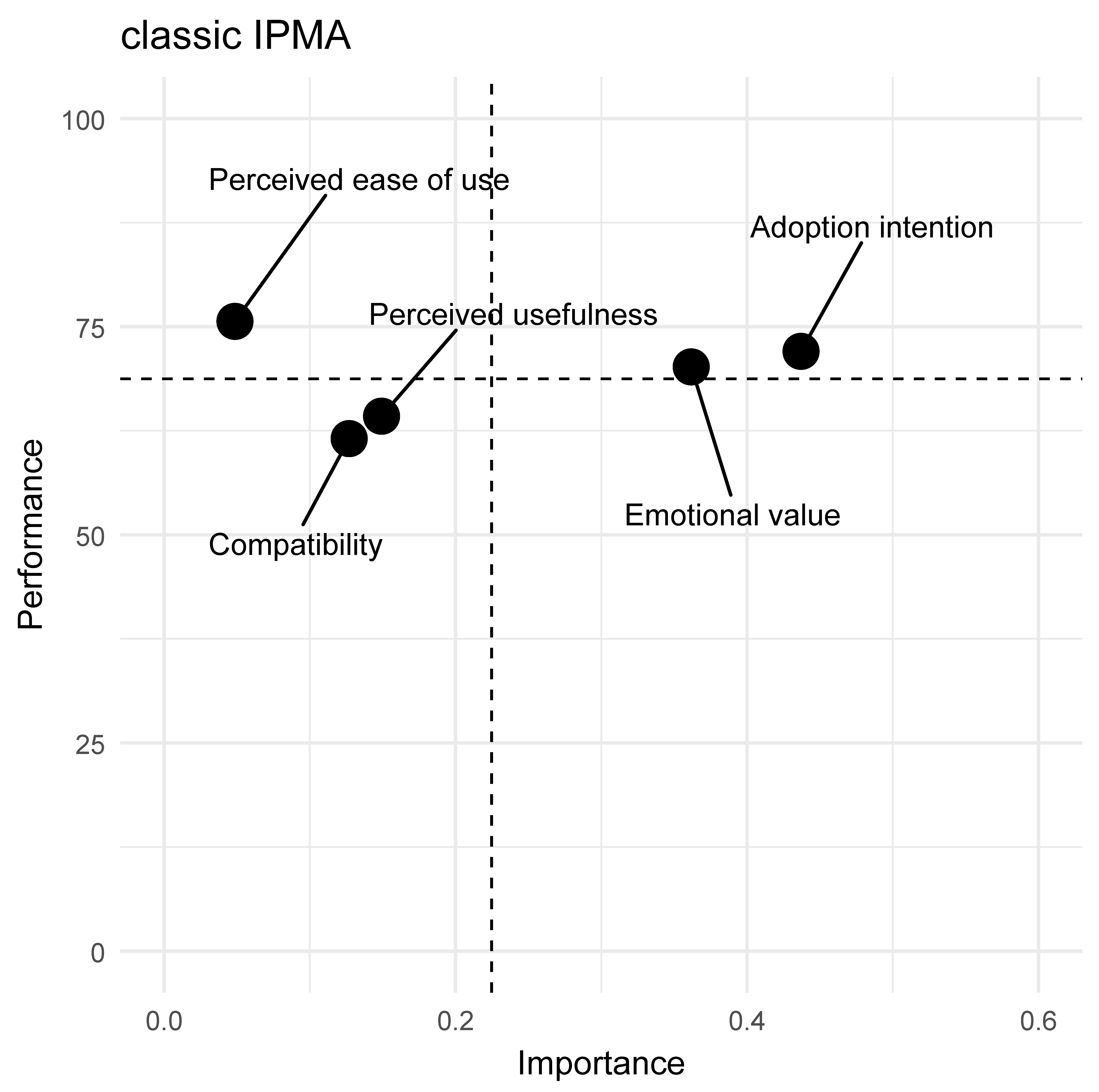
Figure H.2: Classic Importance Performance Map Analysis (IPMA) for the outcome Technology use.
cIPMA adds the bottleneck dimension to IPMA. In selecting the priority predictor, cIPMA not only considers the Importance and Performance scores of the predictor, but also the percentage of bottleneck cases of the predictor: the percentage of cases that are unable to achieve a particular target outcome level. As shown above, the percentage of bottleneck cases per predictor can be obtained with the helper function get_bottleneck_cases. To produce cIPMA, the IPMA dataset with Importance and Performance scores is extended with the percentage of bottleneck cases. The function get_cipma_df is used for this. Note that the output includes the column ‘Necessity’ that indicates whether the predictor is necessary given the selected threshold values for the effect size \(d\) and the \(p\)-value. These predictors should not show up in the bottleneck table and therefore should not be part of cIPMA’s bottleneck dimension. Therefore, in the get_cipma_df helper function a standard point size as in IPMA is given to such predictors. This R function can be downloaded from the book-page: https://jandul.github.io/NCA.
# cIPMA  - dataset
source("get_cipma_df.R")
d_threshold <- 0.10
p_threshold <- 0.05
model <- model1.technology

# Extract parameters
effect_size <- sapply(predictors, nca_extract, model = model, ceiling = "ce_fdh",
                      param   = "Effect size")
p_value <- sapply(predictors, nca_extract, model = model, ceiling = "ce_fdh",
                  param   = "p-value")

necessity <- ifelse(effect_size >= d_threshold & p_value <= p_threshold,
                    "yes", "no")
ipma_df <- IPMA_df_technology
bottlenecks <- bottlenecks_technology
CIPMA_df_technology <- get_cipma_df(ipma_df = ipma_df,
                                    bottlenecks = bottlenecks,
                                    necessity = necessity)
CIPMA_df_technology
## predictor Importance Performance Bottleneck_cases_per
## 1 Perceived usefulness 0.14921041 64.24785 47.126437
## 2 Compatibility 0.12699788 61.55690 8.620690
## 3 Perceived ease of use 0.04863022 75.64040 28.735632
## 4 Emotional value 0.36169649 70.17135 5.747126
## 5 Adoption intention 0.43705233 72.04067 39.080460
## Bottleneck_cases_num Necessity Predictor_with_cases
## 1 82 yes Perceived usefulness (47%, n=82)
## 2 15 yes Compatibility (9%, n=15)
## 3 50 yes Perceived ease of use (29%, n=50)
## 4 10 yes Emotional value (6%, n=10)
## 5 68 yes Adoption intention (39%, n=68)The plot can then be produced with the helper function get_cipma_plot. This R function can be downloaded from the book-page: https://jandul.github.io/NCA.
# cIPMA  - plot
source("get_cipma_plot.R")
cipma_df <- CIPMA_df_technology
x_range <- c(0,0.6)
y_range <- c(0,100)
size_limits = c(0,100)
size_range <- c(0.5,50) # the size of the bulbs
name_plot <- "Original"
cIPMA_plot_technology <- get_cipma_plot(cipma_df = cipma_df,
                                        x_range = x_range,
                                        y_range = y_range,
                                        size_limits = size_limits,
                                        size_range = size_range)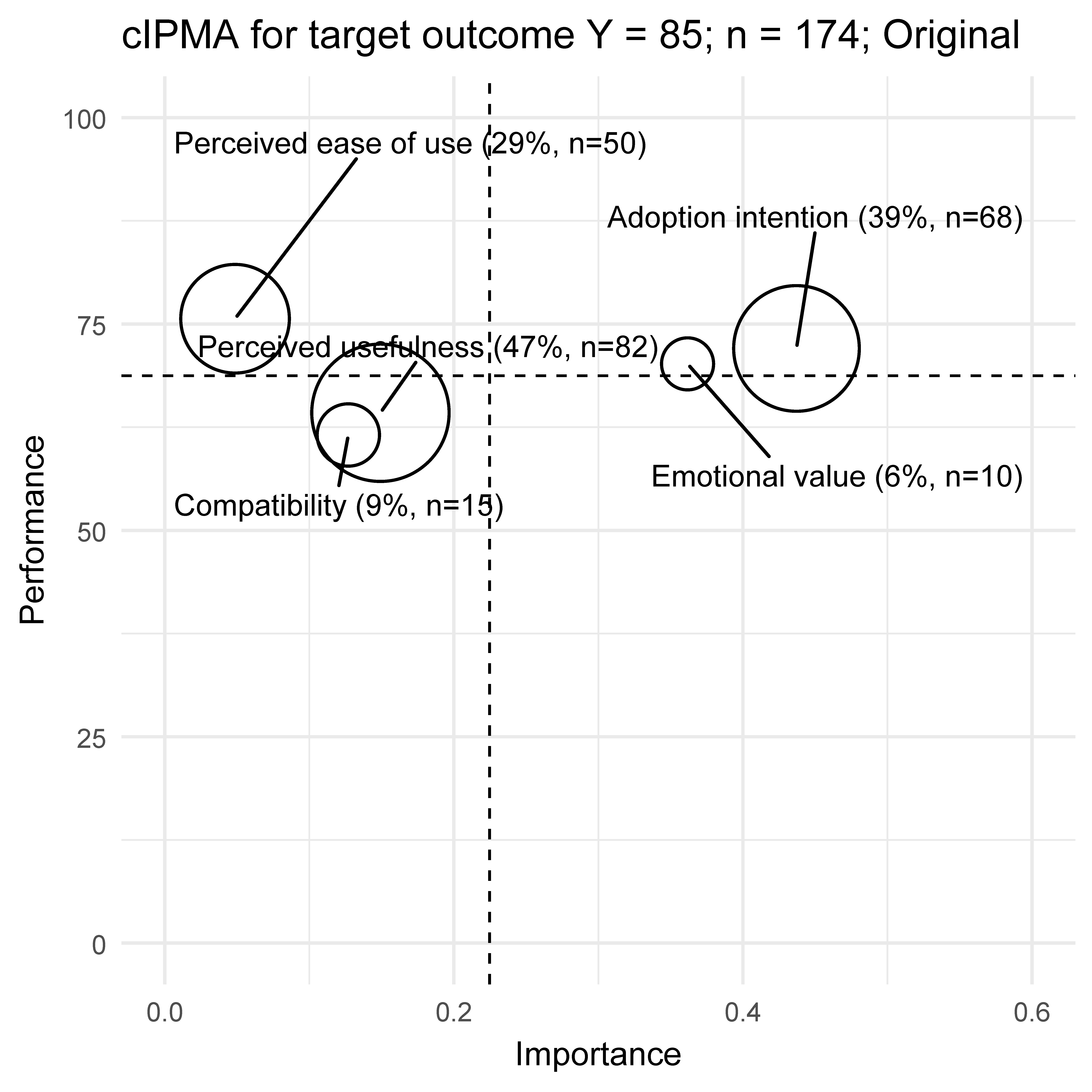
Figure H.3: Combined Importance Performance Map Analysis (cIPMA) for the outcome Technology use. The size of the dot is an indication of the number of cases that cannot achieve the target outcome of 85% of maximum outcome.
The results are shown in Figure H.3, which corresponds to the plots in Hauff et al. (2024) and Sarstedt et al. (2024). The IPMA plot is extended with point sizes that depend on the number or percentage of bottleneck cases. Since all predictors are necessary, each point’s size is relevant. The percentage and number of bottleneck cases are included here between brackets. The NCA results show large differences in percentage and number of bottleneck cases between the five conditions. The order from high to low percentages is: Perceived usefulness, Adoption intention, Perceived ease of use, Compatibility and Emotional value. Perceived usefulness has 47% bottleneck cases, whereas Emotional value has only 6%. This means that from the perspective of NCA, Perceived usefulness is a more relevant than emotional value for a single predictor action. Successful interventions on a single condition (with the goal of bringing all bottleneck cases to at least the threshold level such that the target outcome is possible) will reduce more bottleneck cases when the intervention focuses on Perceived usefulness, rather than on emotional value. Note that such an intervention to eliminate bottlenecks does not guarantee that the target outcome level (85%) will be achieved: a necessary condition for an outcome is not a sufficient condition for it. Additionally, cases may be bottlenecks in multiple conditions. Note also the relevance of a necessary condition in terms of effect size may differ from the relevance of a necessary condition in terms of number of bottleneck cases. The first refers to the magnitude of the constraining role of the condition for the outcome in general, whereas the second refers to the size of the group of cases that cannot achieve a certain target level of the outcome. For emotional value the effect size is largest (0.33), but the percentage of bottleneck cases is lowest (6%).
The BIPMA extends the cIPMA by considering only single bottleneck cases per predictor as explained in Section 11.4.1.7. The number of single bottleneck cases can be extracted with the helper function get_single_bottleneck_cases. This R function can be downloaded from the book-page: https://jandul.github.io/NCA.
# Single bottleneck cases - Target outcome 85
source("get_single_bottleneck_cases.R")
data <- dataset1
ceilings = "ce_fdh"
target_outcome <- 85
predicted <- "Technology use"
predictors <-  c("Perceived usefulness",
                 "Compatibility",
                 "Perceived ease of use",
                 "Emotional value",
                 "Adoption intention")
corner = 1 # default expected empty space for all conditions
single_bottlenecks_technology <- get_single_bottleneck_cases(
                                data,
                                conditions = predictors,
                                outcome = predicted,
                                corner = corner,
                                target_outcome=target_outcome,
                                ceiling = ceilings)
single_bottlenecks_technology
## $single_bottleneck_cases_per
## Bottlenecks (Y = 85)
## Perceived usefulness 14.9425287
## Compatibility 0.5747126
## Perceived ease of use 4.0229885
## Emotional value 0.0000000
## Adoption intention 8.0459770
##
## $single_bottleneck_cases_num
## Bottlenecks (Y = 85)
## Perceived usefulness 26
## Compatibility 1
## Perceived ease of use 7
## Emotional value 0
## Adoption intention 14
##
## $threshold
## Perceived usefulness Compatibility Perceived ease of use
## 66.21236 33.69644 66.90439
## Emotional value Adoption intention
## 49.65026 75.00000
##
## $single_bottleneck_case_names
## $single_bottleneck_case_names$`Perceived usefulness`
## [1] "15" "26" "32" "44" "49" "51" "62" "68" "71" "73" "78" "91"
## [13] "92" "94" "101" "102" "113" "115" "118" "126" "138" "152" "162" "163"
## [25] "164" "166"
##
## $single_bottleneck_case_names$Compatibility
## [1] "109"
##
## $single_bottleneck_case_names$`Perceived ease of use`
## [1] "7" "24" "40" "45" "65" "79" "105"
##
## $single_bottleneck_case_names$`Emotional value`
## character(0)
##
## $single_bottleneck_case_names$`Adoption intention`
## [1] "11" "23" "25" "27" "38" "39" "74" "85" "89" "106" "110" "136"
## [13] "140" "157"
##
##
## $any_bottleneck_case_names
## [1] "1" "2" "6" "7" "8" "9" "11" "14" "15" "19" "20" "22"
## [13] "23" "24" "25" "26" "27" "28" "29" "31" "32" "36" "38" "39"
## [25] "40" "42" "43" "44" "45" "47" "48" "49" "50" "51" "52" "54"
## [37] "56" "58" "61" "62" "64" "65" "68" "70" "71" "73" "74" "78"
## [49] "79" "83" "85" "86" "88" "89" "90" "91" "92" "94" "95" "96"
## [61] "97" "101" "102" "103" "105" "106" "108" "109" "110" "111" "113" "114"
## [73] "115" "116" "117" "118" "119" "120" "121" "122" "123" "124" "125" "126"
## [85] "132" "134" "135" "136" "138" "140" "141" "142" "143" "146" "148" "150"
## [97] "151" "152" "153" "157" "158" "160" "162" "163" "164" "166" "168" "169"
## [109] "171" "172" "173" "174"Next, the significant predictor variables for the predicted variable must be identified:
# Significant total effects (SEM)
sem_sig <- TAM_sig
for_select_predicted <- sem_sig[sem_sig$Predicted == predicted, ]
sufficiency <- ifelse(for_select_predicted$Sig_Total, "yes", "no")
names(sufficiency) <- predictors
The BIPMA dataset with Bottlenecks (single bottlenecks), Importance and Performance scores can be obtained with the helper function get_bipma_df. This R function can be downloaded from the book-page: https://jandul.github.io/NCA.
# BIPMA  - dataset
source("get_bipma_df.R")
ipma_df <- IPMA_df_technology
single_bottlenecks <- single_bottlenecks_technology
BIPMA_df_technology <- get_bipma_df(ipma_df = ipma_df,
                                    single_bottlenecks=single_bottlenecks,
                                    necessity = necessity,
                                    sufficiency = sufficiency)
BIPMA_df_technology
## predictor Importance Performance Single_bottleneck_cases_per
## 1 Perceived usefulness 0.14921041 64.24785 14.9425287
## 2 Compatibility 0.12699788 61.55690 0.5747126
## 3 Perceived ease of use 0.04863022 75.64040 4.0229885
## 4 Emotional value 0.36169649 70.17135 0.0000000
## 5 Adoption intention 0.43705233 72.04067 8.0459770
## Single_bottleneck_cases_num Necessity Corner Target_outcome Sufficiency
## 1 26 yes 1 85 no
## 2 1 yes 1 85 no
## 3 7 yes 1 85 no
## 4 0 yes 1 85 yes
## 5 14 yes 1 85 yes
## Predictor_with_single_cases
## 1 Perceived usefulness (15%, n=26)
## 2 Compatibility (1%, n=1)
## 3 Perceived ease of use (4%, n=7)
## 4 Emotional value (0%, n=0)
## 5 Adoption intention (8%, n=14)The BIPMA can be created with the helper function get_bipma_plot. This R function can be downloaded from the book-page: https://jandul.github.io/NCA.
# Bipma - plot
source("get_bipma_plot.R")
bipma_df <- BIPMA_df_technology
x_range <- c(0,0.6)
y_range <- c(0,100)
size_limits = c(0,100)
size_range <- c(0.5,50) # the size of the bulbs
BIPMA_plot_technology <- get_bipma_plot(bipma_df = bipma_df,
                                        x_range = x_range,
                                        y_range = y_range,
                                        size_limits = size_limits,
                                        size_range = size_range)
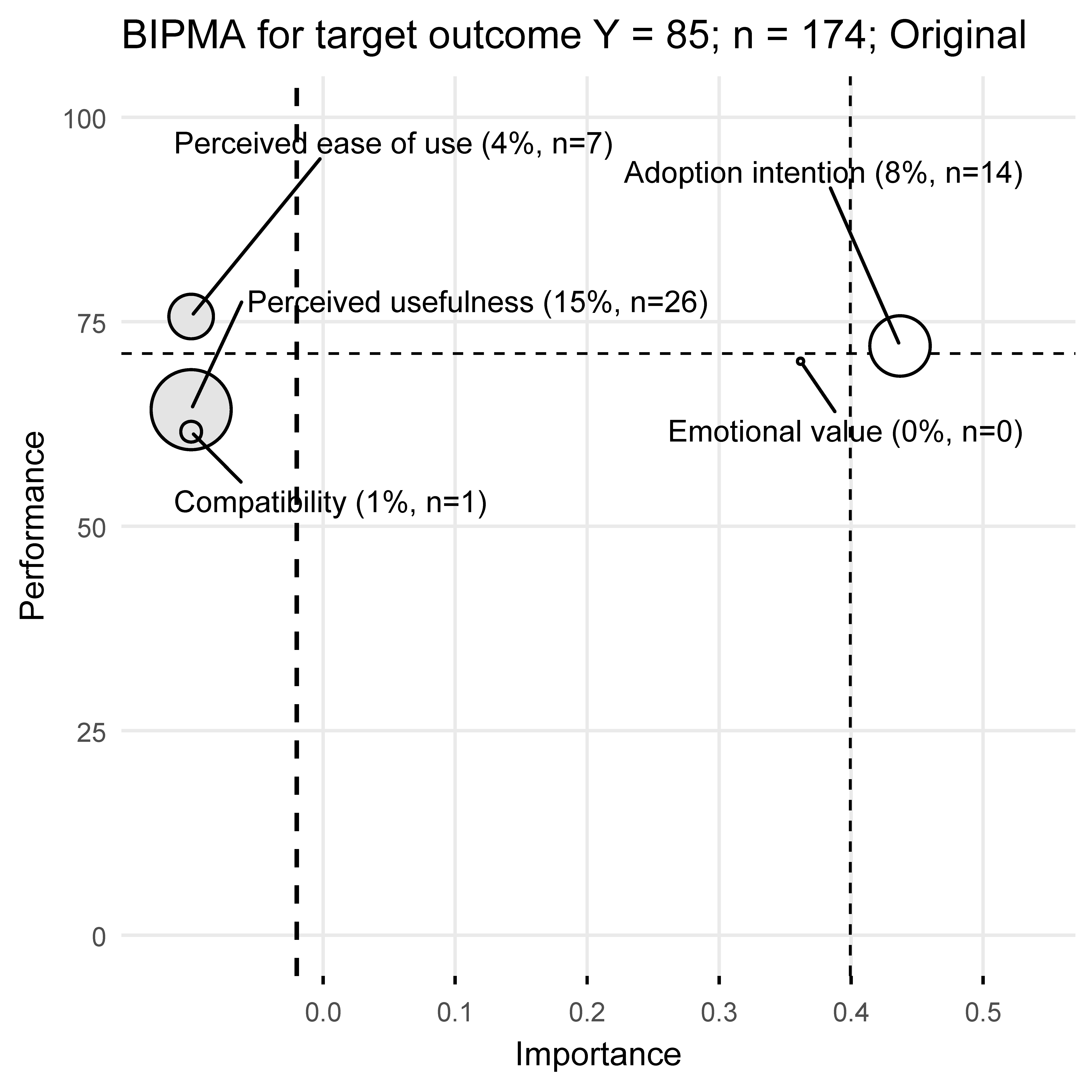
Figure H.4: Bottleneck Importance Performance Map Analysis (BIPMA) for the outcome Technology use. The size of the dot is an indication of the number of single bottleneck cases that cannot achieve the target outcome of 85% of maximum outcome. White dot: Significant average effect and significant necessity effect. Gray dot: Non-significant average effect and significant necessity effect. The horizontal and vertical thin dashed lines correspond to mean Performance and the mean Importance of the predictors with a significant total average effect, respectively.
The results are shown in Figure H.4. For each condition the percentage and number of single bottleneck cases is given between brackets. The results again show large differences in the percentage and number of single bottleneck cases between the five conditions. In this case, the order from high to low percentages is the same as for cIPMA as shown in Figure H.3. However, the number and percentage of bottleneck cases are in BIPMA considerably lower than in cIPMA. Perceived usefulness has most single bottleneck cases (15%, n=26), whereas Emotional value has none. This means that, in contrast to the conclusion from cIPMA, emotional value is not a relevant predictor for an action based on NCA if only one condition can be changed. Successful group interventions on a single predictor (with the goal to bring all bottleneck cases above the threshold level) could focus on Perceived usefulness, which has almost twice as many single bottlenecks as Adoption intention. Perceived usefulness, Compatibility and Perceived ease of use have non-significant average effects on Technology use according to SEM. Predictors that are necessary from the perspective of NCA, but are non-significant predictors from the perspective of SEM, are placed on the Importance axis to the left of Importance = 0 and the corresponding points are shown in gray. Predictors that are significant from the perspective of SEM but non-significant from the perspective of NCA are shown as small black points, but none of the conditions in this analysis were non-significant from the perspective of NCA. Note, that it is possible that a condition without bottleneck cases is also displayed this way (Emotional value), but such a condition is irrelevant for an NCA-based intervention. Predictors that are non-significant from the perspective of both SEM and NCA are separately mentioned in the BIPMA plot in a text box (Figure 11.5) to indicate that actions on such predictors are not effective. However, in the TAM example non-significant predictors from the necessity perspective were not identified.
For selecting a proper group intervention strategy based on the BIPMA results, see Section 11.4.1.7. For a selecting a case-specific interventions strategy based only on the NCA results, see Chapter 12.
H.8 Step 8: Interpret results
The results of the SEM study suggest that for increasing the Technology use on average, only Emotional value and Adoption intention are effective. At the same time, the NCA study shows that a high level of Technology use is only achievable when all predictors meet a certain minimum level. To evaluate the robustness of these NCA results several checks can be done (Section 9.12). Robustness checks for SEM are not discussed here. For this demonstration eight checks are selected (Table H.3). In each check, one choice is changed and the new results are compared with the original results, and it is evaluated if the conclusion regarding necessity is changed.
The type of changes in several analyst’s choices regarding necessity is shown in Table H.3.
| Robustness check | Original | Ceiling change | d-threshold change | p-threshold change | Scope change | Single outlier removal | Multiple outlier removal | Target lower | Target higher |
|---|---|---|---|---|---|---|---|---|---|
| Ceiling line | CE-FDH | CR-FDH | CE-FDH | CE-FDH | CE-FDH | CE-FDH | CE-FDH | CE-FDH | CE-FDH |
| Threshold effect size | 0.10 | 0.10 | 0.20 | 0.10 | 0.10 | 0.10 | 0.10 | 0.10 | 0.10 |
| Threshold p-value | 0.05 | 0.05 | 0.05 | 0.01 | 0.05 | 0.05 | 0.05 | 0.05 | 0.05 |
| Scope | empirical | empirical | empirical | empirical | theoretical | empirical | empirical | empirical | empirical |
| Outliers | no | no | no | no | no | yes, single | yes, multiple | no | no |
| Target outcome | 85 | 85 | 85 | 85 | 85 | 85 | 85 | 80 | 90 |
The results of these robustness checks for each individual predictor variable are shown in the following set of tables:
Predictor: Perceived usefulness
| Robustness check | Effect size | p-value | Necessity | Single bottlenecks (%) | Single bottlenecks (n) | Priority |
|---|---|---|---|---|---|---|
| Original | 0.24 | < 0.001 | yes | 14.9 | 26 | 1/5 |
| Ceiling line change | 0.19 | 0.001 | yes | 5.2 | 9 | 2/5 |
| Effect size thresh. change | 0.24 | < 0.001 | yes | 14.9 | 26 | 1/5 |
| Significance level change | 0.24 | < 0.001 | yes | 14.9 | 26 | 1/5 |
| Scope change | 0.24 | < 0.001 | yes | 14.9 | 26 | 1/5 |
| Outlier change 1 | 0.30 | < 0.001 | yes | 6.5 | 11 | 1/5 |
| Outlier change 2 | 0.29 | < 0.001 | yes | 6.6 | 11 | 1/5 |
| Target outcome lower | 0.24 | < 0.001 | yes | 10.3 | 18 | 1/5 |
| Target outcome higher | 0.24 | < 0.001 | yes | 14.9 | 26 | 1/5 |
Predictor: Compatibility
| Robustness check | Effect size | p-value | Necessity | Single bottlenecks (%) | Single bottlenecks (n) | Priority |
|---|---|---|---|---|---|---|
| Original | 0.21 | < 0.001 | yes | 0.6 | 1 | 4/5 |
| Ceiling line change | 0.15 | < 0.001 | yes | 2.3 | 4 | 3/5 |
| Effect size thresh. change | 0.21 | < 0.001 | yes | 0.6 | 1 | 4/5 |
| Significance level change | 0.21 | < 0.001 | yes | 0.6 | 1 | 4/5 |
| Scope change | 0.21 | < 0.001 | yes | 0.6 | 1 | 4/5 |
| Outlier change 1 | 0.28 | < 0.001 | yes | 1.2 | 2 | 5/5 |
| Outlier change 2 | 0.29 | < 0.001 | yes | 1.2 | 2 | 5/5 |
| Target outcome lower | 0.21 | < 0.001 | yes | 1.1 | 2 | 3/5 |
| Target outcome higher | 0.21 | < 0.001 | yes | 0.6 | 1 | 4/5 |
Predictor: Perceived ease of use
| Robustness check | Effect size | p-value | Necessity | Single bottlenecks (%) | Single bottlenecks (n) | Priority |
|---|---|---|---|---|---|---|
| Original | 0.24 | 0.015 | yes | 4.0 | 7 | 3/5 |
| Ceiling line change | 0.20 | 0.013 | yes | 1.7 | 3 | 4/5 |
| Effect size thresh. change | 0.24 | 0.015 | yes | 4.0 | 7 | 3/5 |
| Significance level change | 0.24 | 0.015 | no | 4.0 | 7 | 3/5 |
| Scope change | 0.36 | 0.015 | yes | 4.0 | 7 | 3/5 |
| Outlier change 1 | 0.18 | 0.047 | yes | 3.0 | 5 | 3/5 |
| Outlier change 2 | 0.13 | 0.051 | no | 3.0 | 5 | 3/5 |
| Target outcome lower | 0.24 | 0.015 | yes | 0.6 | 1 | 5/5 |
| Target outcome higher | 0.24 | 0.015 | yes | 4.0 | 7 | 3/5 |
Predictor: Emotional value
| Robustness check | Effect size | p-value | Necessity | Single bottlenecks (%) | Single bottlenecks (n) | Priority |
|---|---|---|---|---|---|---|
| Original | 0.33 | < 0.001 | yes | 0.0 | 0 | 5/5 |
| Ceiling line change | 0.17 | 0.020 | yes | 0.0 | 0 | 5/5 |
| Effect size thresh. change | 0.33 | < 0.001 | yes | 0.0 | 0 | 5/5 |
| Significance level change | 0.33 | < 0.001 | yes | 0.0 | 0 | 5/5 |
| Scope change | 0.33 | < 0.001 | yes | 0.0 | 0 | 5/5 |
| Outlier change 1 | 0.44 | < 0.001 | yes | 2.4 | 4 | 4/5 |
| Outlier change 2 | 0.44 | < 0.001 | yes | 2.4 | 4 | 4/5 |
| Target outcome lower | 0.33 | < 0.001 | yes | 1.1 | 2 | 3/5 |
| Target outcome higher | 0.33 | < 0.001 | yes | 0.0 | 0 | 5/5 |
Predictor: Adoption intention
| Robustness check | Effect size | p-value | Necessity | Single bottlenecks (%) | Single bottlenecks (n) | Priority |
|---|---|---|---|---|---|---|
| Original | 0.29 | < 0.001 | yes | 8.0 | 14 | 2/5 |
| Ceiling line change | 0.20 | 0.001 | yes | 5.7 | 10 | 1/5 |
| Effect size thresh. change | 0.29 | < 0.001 | yes | 8.0 | 14 | 2/5 |
| Significance level change | 0.29 | < 0.001 | yes | 8.0 | 14 | 2/5 |
| Scope change | 0.29 | < 0.001 | yes | 8.0 | 14 | 2/5 |
| Outlier change 1 | 0.38 | < 0.001 | yes | 5.3 | 9 | 2/5 |
| Outlier change 2 | 0.42 | < 0.001 | yes | 5.4 | 9 | 2/5 |
| Target outcome lower | 0.29 | < 0.001 | yes | 1.7 | 3 | 2/5 |
| Target outcome higher | 0.29 | < 0.001 | yes | 8.0 | 14 | 2/5 |
Without discussing details, the general results of the NCA robustness tables are as follows. The results for the necessity of Perceived usefulness are robust with respect to the conclusion about necessity-in-kind. For necessity-in-degree only a change of ceiling line from CE-FDH to CR-FDH resulted in a different priority level (from first to second). Most single bottleneck cases exist for this predictor. Generally, the original results for this predictor can be considered as robust. The same conclusion applies to Compatibility. The original conclusion about necessity-in-kind is stable and for all checks the priority level for action remains low. However, the results of Perceived ease of use are more variable. For example, the statistical significance of the original finding and therefore the conclusion of necessity is somewhat fragile. Also the number of bottleneck cases changes from 7 to 1 and is sensitive to small changes of the selected target level. The results for Emotional value and Adoption intention are relatively robust.
Note that the NCA robustness table is a tool for better understanding and communicating the credibility of the original results. The findings from the checks largely depend on the selected parameters for the checks. No hard rules exist to decide about the robustness or fragility of the results, as this is a judgement by the analyst and others.