2 Causality

2.1 Summary of this chapter

NCA uses a causal perspective that is (partly) different from common views on causality. This chapter presents NCA’s causal perspective by comparing it to other causal perspectives. The chapter begins by discussing what a cause is (Section 2.2), followed by a discussion of the commonly used sufficiency causality (Section 2.3). Next, necessity causality is discussed (Section 2.4). For both types of causality, three perspectives are distinguished: deterministic, probabilistic, and typicality (deterministic with exceptions). NCA uses the deterministic (or typicality) necessity causal perspective. In the next section (Section 2.5), NCA’s use of conditional logic (assuming a causal direction) is compared with the conventional view on conditional logic (in which no causal direction is assumed). Subsequently, another unique feature of NCA is discussed: the concept of necessary condition in degree (NiD), which extends the conventional binary approach (absence or presence of $X$ is necessary for absence or presence of $Y$) to a continuous approach: level $x$ of $X$ is necessary for level $y$ of $Y$ (Section 2.6). Finally, Section 2.7 discusses that, due to causal underdetermination, no causal perspective is superior to another.

2.2 What is a cause?

Causality is often loosely defined as the influence of a cause $X$ on an effect $Y$. General expressions like $X$ has an effect on $Y$, $X$ affects $Y$, or $X$ contributes to $Y$ without specifying the type of causality are commonplace. Causality is a complex subject that is extensively debated in the philosophy of science literature and elsewhere. The Scottish philosopher David Hume (1711–1776) laid the foundation for modern discussions about causation. Hume defined a cause as follows:

“… we may define a cause to be an object, follow’d by another, and where all the objects, similar to the first, are follow’d by objects, similar to the second: Or in other words, where, if the first object had not been, the second never had existed” (Hume, 1756, p. 121)

The first part of this definition refers to sufficiency causality (if $X$, then $Y$).¹⁰ It includes a specification of the temporal order: $Y$ follows $X$, and a generalization: the statement applies also to “similar objects.” The second part of the definition refers to necessity causality (if not $X$, then not $Y$)¹¹ although without the generalization (for a further discussion see Dul, 2024a). The two types of causality are illustrated in Figure 2.1, showing observed $XY$ patterns where $X$ is the condition and $Y$ is the outcome that can have two values (absent/present).¹² When $X$ is a sufficient cause for $Y$ (Figure 2.1-left), observations (points, cases) can exist in all corners except corner 4: If $X$ is present, then $Y$ is present. When $X$ is a necessary cause for $Y$ (Figure 2.1-right), observations can exist in all corners except in corner 1: If $X$ is absent, then $Y$ is absent. The corner where observations are not possible is called the empty space and the corner where observations are possible is called the feasible area.

$XY$-tables illustrating sufficiency causality (Left) and necessity causality (Right) with binary concepts. Gray = observations (points, cases) are possible. White = no observations are possible.

Figure 2.1: $XY$-tables illustrating sufficiency causality (Left) and necessity causality (Right) with binary concepts. Gray = observations (points, cases) are possible. White = no observations are possible.

2.3 Sufficiency causality

Most phenomena in the social, biomedical, and other sciences are studied from the perspective of sufficiency causality (if $X$, then $Y$). When people talk about a cause or causality, they (almost always) implicitly mean sufficiency causality.

Three fundamentally different perspectives on sufficiency causality can be distinguished: deterministic, probabilistic, and typicality (Dul, 2024a). Table 2.1 summarizes these perspectives and lists some main methods that (implicitly) use this perspective when inferring causality.

Table 2.1: Perspectives on sufficiency causality: if $X$, then … $Y$.
Perspective	Logic	Main methods
Deterministic	if X, then Y	QCA, SCC, NESS
Probabilistic	if X, then Y	LR, MLR, SEM
Typicality	if X, then Y	Methods in physics
Note:
QCA = Qualitative Comparative Analysis
SCC = Sufficient Component Cause
NESS = Necessary Element of a Sufficient Set
LR = Logistic (Logit) Regression
MLR = Multiple Linear Regression
SEM = Structural Equation Modeling

2.3.1 Deterministic sufficiency

Hume’s sufficiency definition has been interpreted as being about deterministic causality: if $X$, then always $Y$ (e.g., Baumgartner, 2009). Many phenomena in the physical world may be described by such a deterministic sufficiency causal perspective. For example, reaching the speed of sound produces a sonic boom. In the social sciences, single deterministic sufficiency causes are rare, as normally several factors together produce an outcome. Such a sufficiency perspective is used in ‘parts-whole’ methods and frameworks (Machamer et al., 2000; Varzi, 2019). The Sufficient-Component Cause model in medicine [SCC; Rothman (1976)], the Necessary Element of a Sufficient Set approach in law (NESS, Wright, 1985), and Qualitative Comparative Analysis in social sciences [QCA; Ragin (1987); Campbell & Fiss (2026)], for example, use such a sufficiency perspective. The combination of causal factors (called configurations in QCA) is considered deterministically sufficient for the outcome: If [combination of $X$’s], then $Y$. Several combinations may be sufficient (‘equifinality’), such that none of these configurations is necessary for the outcome. The causal factors that are parts of the configurations are called INUS conditions: Insufficient but Necessary parts of Unnecessary but Sufficient configurations (Mackie, 1965). INUS conditions should not be confused with necessary conditions; INUS conditions are ‘locally’ necessary for the configuration to produce the outcome, and usually not overall necessary for the outcome itself (Dul, Vis, et al., 2021). NCA considers only the overall necessary conditions for the outcome. Although the theoretical foundations of SCC, NESS, and QCA are based on a deterministic ontology, in practice the determinism may be imperfect.¹³ Deterministic sufficiency means that corner 4 of Figure 2.1-left remains empty.

2.3.2 Probabilistic sufficiency

As single deterministic sufficiency causes are rare in the social sciences, a non-deterministic causal approach is often adopted: probabilistic sufficiency: ‘if $X$, then probably $Y$’, or ‘if $X$, then likely $Y$.’ Pearl states that:

“According to one of the basic tenets of probabilistic causality, a cause should raise the probability of the effect” (Pearl, 2009, p. 254)

The dominant framework of the probabilistic sufficiency causal perspective focuses on the average effects of ‘parts’ of the whole. The lower-right corner is not empty but is less populated than the other cells. It identifies the Average Causal Effect (ACE) or Average Treatment Effect (ATE) of a causal factor. The approach is currently mainstream in quantitative studies using statistical methods. Statistical models are based on the assumption of the probability distributions of the cause and the effect. The effect is produced by an unknown ‘data generation process’ that describes the underlying relationships between concepts and the stochastic processes involved in generating the observed data. When statistical models with regression-based methods are used to infer causality, the underlying causal perspective is probabilistic sufficiency. Examples of regression-based methods that are commonly used for inferring causality are multiple linear regression (MLR), logistic (logit) regression, and structural equation modeling (SEM). Probabilistic sufficiency may be inferred if the lower-right corner of $XY$-tables or $XY$-plots is less densely populated with observations than the other corners (Figures 2.1 and 2.3).

2.3.3 Typicality sufficiency

A recently developed non-deterministic and non-probabilistic perspective on causality is the ‘typicality’ perspective. The typicality sufficiency causal perspective was introduced in physics, including quantum mechanics and thermodynamics (e.g., Goldstein, 2012; Wilhelm, 2022). It challenges the deterministic ontology but does not adopt a probabilistic ontology. The typicality interpretation also gets attention in other scientific disciplines, including the social sciences (Wagner, 2020). This perspective can be described as deterministic with exceptions. It accepts the perspective if $X$, then $Y$ but fundamentally allows exceptions: if $X$, then typically $Y$, or if $X$, then almost always $Y$. The typicality perspective does not describe exceptions in terms of likelihood of occurrence, but in terms of cardinality (Wilhelm, 2022): the number of elements that deviates from the majority of the elements in the set. Typicality sufficiency means that corner 4 of Figure 2.1-left remains empty, but a few observations may be exceptions.

2.4 Necessity causality

The three types of perspectives on causality can also be applied to necessity causality. This is shown in Table 2.2.

2.4.1 Deterministic necessity

The second sentence of Hume’s definition of causality can be considered a deterministic view on necessity causality (Goertz & Mahoney, 2012). If $X$ does not occur, $Y$ will not happen. Whereas single sufficient causes are seldom on their own sufficient for an effect, single necessity causes alone can stop an effect from occurring if absent. For example, oxygen is necessary for human life but not sufficient on its own. There are multiple necessity causes for human life, and each will stop the outcome from occurring if it is absent. Deterministic necessity means that corner 1 of Figure 2.1-right remains empty.

2.4.2 Probabilistic necessity

The probabilistic necessity perspective can be phrased as: If not $X$, then probably not $Y$. Probabilistic necessity means that corner 1 of Figure 2.1-right may have observations but is less densely populated than the other corners.

2.4.3 Typicality necessity

The idea of typicality was developed for sufficiency causality but can also be applied to necessity causality (Dul, 2024a). It accepts a deterministic perspective with exceptions: if not $X$, then typically not $Y$, or if not $X$, then almost always not $Y$. Again, the typicality perspective does not describe exceptions in terms of probabilities but in terms of cardinality. Typicality necessity means that corner 1 of Figure 2.1-right remains empty, but a few observations may be exceptions. Exceptions are rare without quantifying what is “rare.” If an exception is not an error, it could be a unique counterexample (e.g., an innovative case), worth studying in detail. However, the phenomenon of interest is still described with deterministic necessity, excluding the exception.¹⁴ Note that NCA has a deterministic view on causality and that the ceiling line is a sharp border between an area with cases and an area without cases (Section 4.3.2). The presence of outliers (in the “empty” space) indicates that necessity does not exist, rather than that necessity exists with high probability.

With a deterministic view on necessity causality, a case with high $Y$ and low $X$ rejects necessity. The data point may be mistakenly in the empty area because of measurement error, sampling, or case selection error. Such errors may be corrected, or the case may be removed from further consideration if the error cannot be repaired. However, if the case is not an error it may be a special case: a rare exception in the otherwise empty space, representing another phenomenon not captured by necessity. Only the presence of such exception may be the reason for adopting the typicality perspective. NCA keeps its deterministic approach, but allows rare exceptions. Having many outlier cases in the “empty” space that cannot be explained by errors is a reason to reject necessity (or to redefine the formal hypothesis; see Chapter 7 if these cases have a common characteristic), but it is not a reason to accept necessity with a lenient view on (typicality) necessity.

Table 2.2: Perspectives on necessity causality: if not $X$, then … not $Y$.
Perspective	Logic	Main methods
Deterministic	if not X, then not Y	NCA, (QCA)
Probabilistic	if not X, then not Y	(PN)
Typicality	if not X, then not Y	NCA
Note:
NCA = Necessary Condition Analysis
QCA = Qualitative Comparative Analysis (only in kind; typicality implicit)
PN = Probability of Necessity (only binary variables; no generic necessity)

Table 2.2 maps different methods on the three causal perspectives. It shows that NCA can be used for the deterministic and typicality perspectives. The table also includes QCA for identifying necessity using a deterministic or typicality perspective. Although QCA’s main focus is on sufficiency, and QCA studies often ignore necessity, QCA can also identify necessity. The necessity analysis of QCA is less detailed than that of NCA, as it only identifies necessity-in-kind (NiK)¹⁵ and often misses necessary conditions (Torres & Godinho, 2022). The differences between necessity approaches of NCA and QCA are explained in Dul (2016a) and Vis & Dul (2018) and summarized in Section 11.5. The table also mentions Pearl’s Probability of Necessity (PN) approach for identifying probabilistic necessity using a counterfactual analysis. Pearl (2009) introduced the Probability of Necessity (PN) concept (where $X$ and $Y$ are binary) to address the question: “Was event $X$ necessary for event $Y$ to occur?” PN is the probability that $Y$ would not have occurred if $X$ had not occurred, given that both $X$ and $Y$ actually occurred.¹⁶ This is a counterfactual probability conditioned on the actual world where $X$ and $Y$ happened. PN evaluates a hypothetical world where $X$ did not happen. PN is used for identifying necessity causes at the individual level, for example in legal reasoning, where the question is not whether in general $X$ is a probabilistic cause of $Y$, but rather whether $X$ was the necessity cause of $Y$ in a specific situation that has happened.

2.5 Causal versus conditional logic

NCA extends conditional logic with causality. In conditional logic, as used in philosophy and mathematics, relationships are described in terms of if-then statements. In the statement ‘if $A$, then $B$’, $A$ is the antecedent and $B$ is the consequent, and $A$ and $B$ usually have only two values: true or false. The truth or falsity of $B$ depends on the truth or falsity of $A$. In conditional logic, ‘if $A$, then $B$’ means that $A$ implies $B$, or if $A$ occurs, then $B$ occurs. This can be interpreted as $A$ being a sufficient condition for $B$. For example, being born in Italy ($A$) implies having Italian citizenship ($B$). This can be written as:

\[\begin{equation} \tag{2.1} A_s \Rightarrow B \end{equation}\]

Here the subscript ‘$s$’ emphasizes the interpretation of $A$ as a sufficient condition, and the double arrow $\Rightarrow$ means ‘implies’.

In conditional logic, the statement that $A$ is a necessary condition for $B$ implies that $B$ can only be true if $A$ is true: if $B$, then $A$. For example, oxygen is necessary for human life because being alive implies that the person has access to oxygen. Therefore, truth of $B$ (being alive) implies the truth of $A$ (oxygen). This can be written as:

\[\begin{equation} \tag{2.2} B \Rightarrow A_n \end{equation}\]

where the subscript ‘$n$’ emphasizes the necessary condition interpretation of $A$. This can be rewritten as:

\[\begin{equation} \tag{2.3} A_n \Leftarrow B \end{equation}\]

where the double arrow $\Leftarrow$ means “is implied by.”

Because $B$ can only be true when $A$ is true, the falsity of $A$ implies the falsity of $B$. This can be written as:

\[\begin{equation} \tag{2.4} \neg A_n \Rightarrow \neg B \end{equation}\]

\[\begin{equation} \tag{2.5} \neg B \Leftarrow \neg A_n \end{equation}\]

where the symbol $\neg$ indicates negation, or ‘no’ or ‘not’.

Equations (2.2)–(2.5) are four equivalent expressions for $A_n$ being necessary for $B$ from the perspective of conditional logic.

The phrase $B$ implies $A_n$ (2.2) can also be understood as $B$ is sufficient for $A_n$. Therefore, the expression $A_n$ is necessary for $B$ can be written in four equivalent ways:

$A_n$ is necessary for $B$ (oxygen is necessary for being alive).
$B$ is sufficient for $A_n$ (being alive is sufficient for oxygen).
$A_n$ is sufficient for $B$ (no oxygen is sufficient for not being alive).
$B$ is necessary for $A_n$ (not being alive is necessary for no oxygen).

A major difference between necessity in causal logic as used in NCA, and necessity logic as used in conditional logic is that NCA assumes a causal direction between $A_n$ and $B$ whereas conditional logic does not assume such a causal direction. This means that NCA assumes a temporal order: first $A_n$, followed by $B$. Conditional logic is ignorant about whether there is first oxygen and then life or first life and then oxygen. Therefore, NCA’s causal logic can be seen as an extension of conditional logic where a causal direction is assumed between $A_n$ and $B$. This temporal order excludes the possibility of ‘first $B$, then $A_n$’. The assumption of a temporal order may be justified when first the occurrence of $A_n$ is observed and afterwards the occurrence of $B$, or that it is theoretically implausible that $A_n$ occurs after $B$ (see Section 7.5.3 for a further discussion on temporality). It means that when NCA formulates that $A_n$ is a necessary condition for $B$, it is assumed that $A_n$ is a causal necessary condition for $B$. Assuming also no reverse or reciprocal causality (Section 5.7), it implies that only two of the four conditional expressions are causal statements:

Therefore, in NCA the antecedent $A_n$ is considered the necessity cause of the consequent $B$ (the effect). Statements 2 and 4 still apply as logical statements, but not as causal statements, assuming no reverse or reciprocal causality.

To stress that NCA makes a causal assumption about the relationship between antecedent and consequent, the symbols $A$ and $B$ or $P$ and $Q$ that are common in conventional conditional logic, are replaced by the symbols $X$ and $Y$ to express the cause-effect relationship, where $X$ is the cause and $Y$ is the effect. Then the two equivalent causal expressions for a necessity cause are:

\[\begin{equation} \tag{2.6} X \text{ is necessary for } Y \end{equation}\]

\[\begin{equation} \tag{2.7} \neg X \text{ is sufficient for } \neg Y \end{equation}\]

In the remainder of this book, the expression ‘$X$ is a necessary condition for $Y$’ implies that $X$ is a necessity cause of $Y$ and both expressions (2.6) and (2.7) apply. Dul (2016b) refers to expression (2.6) as the ‘necessity formulation’ of the necessary condition and expression (2.7) as the ‘sufficiency formulation’ of the necessary condition. In this book the statement $X$ is necessary for $Y$ is understood in a deterministic or typicality causal perspective: ‘$X$ is always necessary for $Y$’ or ‘$X$ is almost always/typically necessary for $Y$’. Consequently, all or nearly all observations with the outcome $Y$ do have the necessity cause $X$, and all or nearly all observations that do not have the necessity cause $X$ do not have the outcome $Y$.¹⁷

2.6 From binary necessity to continuous necessity

Another extension that NCA introduces to necessity logic involves the levels of condition $X$ and outcome $Y$. Until now, the book considered the levels of $X$ and $Y$ as binary. Only two values are possible: absent or present (like in Figure 2.1-right), 0 or 1, or false or true, etc. This binary approach is common in conditional logic as well as in the SCC, NESS, and QCA methods and frameworks.¹⁸

NCA extends the binary levels of condition and outcome to multiple possible levels by allowing $X$ and $Y$ to be discrete concepts (with a number of finite levels of more than 2) or continuous concepts (with an infinite number of levels) within minimum and maximum bounds of $X$ and $Y$. This has several consequences.

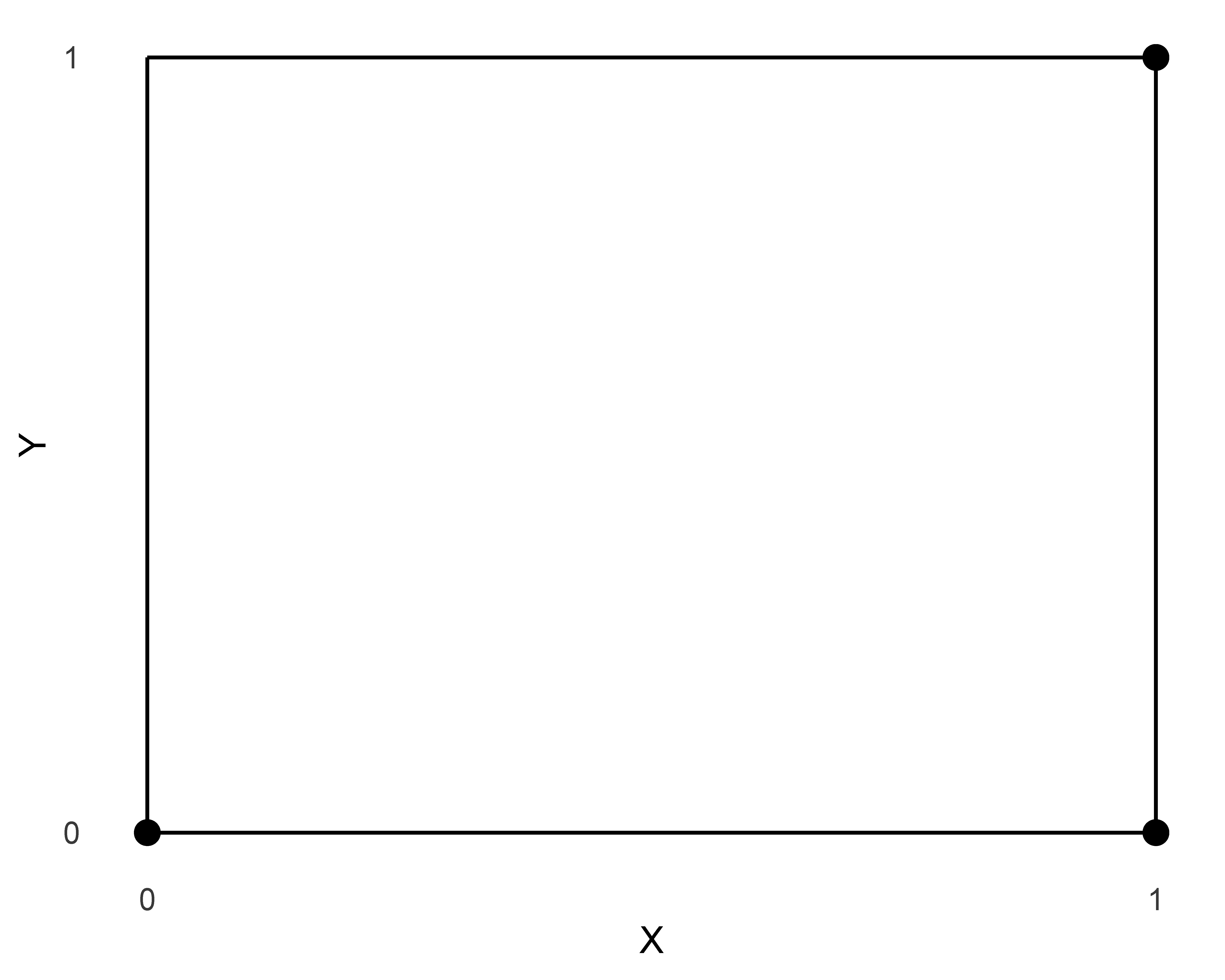
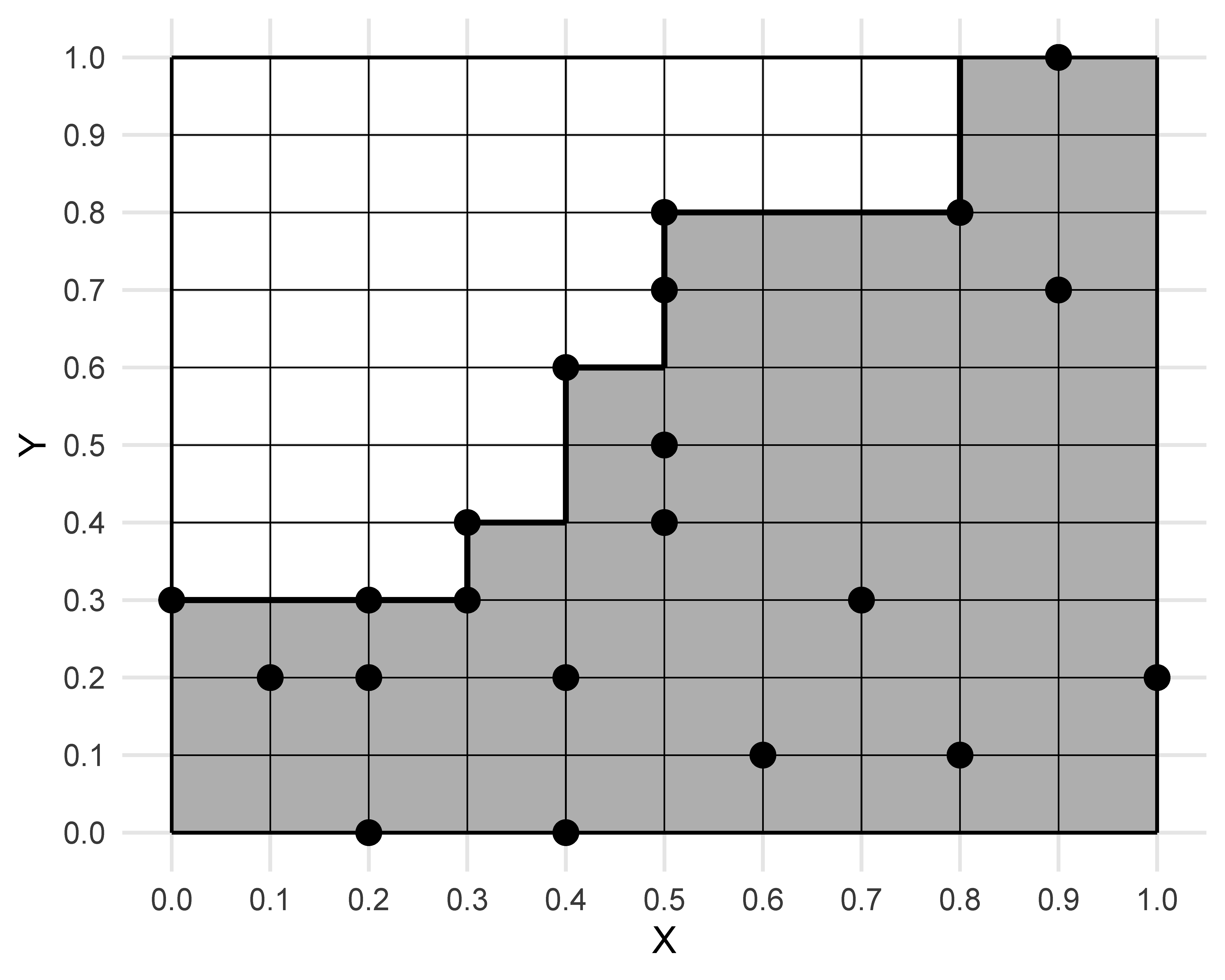
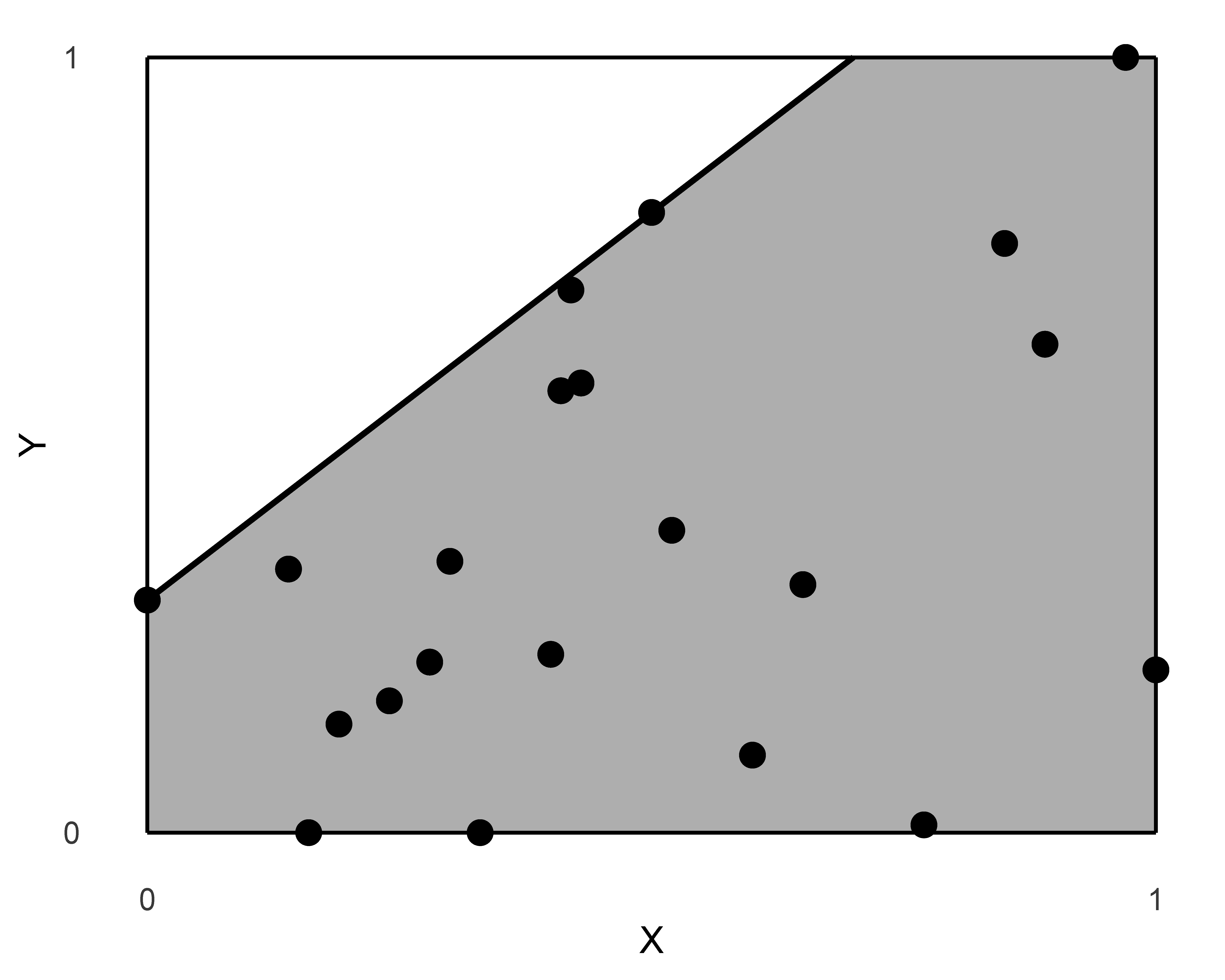
$XY$-plot with dichotomous (Left), discrete (Middle), and continuous (Right) values of condition $X$ and outcome $Y$.

Figure 2.2: $XY$-plot with dichotomous (Left), discrete (Middle), and continuous (Right) values of condition $X$ and outcome $Y$.

First, the $XY$-table is extended to an $XY$-plot as shown in Figure 2.2. Instead of mapping observations on the cells of the $XY$-table, observations are now mapped on a 2D Euclidean coordinate system. The bounds of $X$ and $Y$ are again 0 and 1, but could be any other minimum and maximum values. The bounds on $X$ and $Y$ create a bounding box (Section 4.3). In a dichotomous necessity relationship where both the condition and the outcome are binary, the observations are mapped at corners of the $XY$-plot (Figure 2.2-left). When necessity applies, no observations are possible in the upper-left corner [0,1]. In a discrete necessity relationship observations can be on the intersections of a grid representing the possible discrete values of $X$ and $Y$ (Figure 2.2-middle), and in a continuous necessity relationship observations can exist anywhere in the unit box (Figure 2.2-right), but not in the upper-left corner. Combinations of dichotomous, discrete, and continuous values are also possible in NCA. This is shown in Figure 2.3.

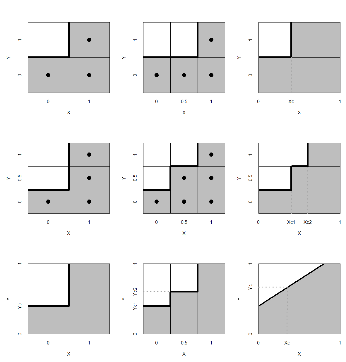
$XY$-plot with combinations of dichotomous, discrete, and continuous values of condition $X$ and outcome $Y$. The upper-left corner is empty if the presence/high value of $X$ is necessary for the presence/high value of $Y$.

Figure 2.3: $XY$-plot with combinations of dichotomous, discrete, and continuous values of condition $X$ and outcome $Y$. The upper-left corner is empty if the presence/high value of $X$ is necessary for the presence/high value of $Y$.

Second, whereas in the dichotomous situation the bounding box $[0,1] × [0,1]$ can be either full or empty, in the discrete and continuous situation it can be partly empty. The size of the empty space may vary, depending on the location of the observations. A border line (ceiling line) separates the empty space (ceiling zone) from the area where observations are possible (feasible area). Referring to the $XY$-plot in Figure 2.2-left where both the condition and the outcome are dichotomous, the ceiling line between empty and feasible area is predefined: the step line connecting the observations [0,0], [0,1], and [1,1] is always the same. The bounding box (unit box) is completely empty, such that points can only be on the ceiling line. No observations can be above or to the left of the ceiling line. In the discrete and continuous situations, the location of the ceiling line depends on the location of the observations in the unit box. This means that the location of the ceiling line and the size of the empty space vary. In any case, there can be no points above or to the left of the ceiling line. If necessity applies, points can only be on, below, or to the right of the ceiling: the feasible area. The ceiling line can be assumed (predefined) or estimated from data. In all situations, the assumption is that the ceiling line represents the sharp border between the empty space and the feasible area to represent deterministic necessity (see model fit measure Sharpness discussed in Section 4.5.6). When a relevant empty space exists that is caused by necessity, the necessary condition is formulated qualitatively as necessity-in-kind (NiK): $X$ is necessary for $Y$.

Third, the discrete and continuous situations add the possibility of a quantitative formulation of a necessary condition statement: level x of $X$ is necessary for level y of $Y$. This is called necessity-in-degree (NiD) and is shown for the continuous situation in Figure 2.4. Any observation $C$ on the ceiling line defines a specific necessity-in-degree: level $X = x_c$ is necessary for level $Y = y_c$. Assuming an increasing ceiling line, the condition must have at least level $x_c$ for outcome level $y_c$. If the condition is less than $x_c$, the outcome will be less than $y_c$. If $X = x_c$, it cannot be concluded that $Y = y_c$, but only that $Y \leq y_c$. This situation can be described by level $x_c$ of $X$ is necessary but not sufficient for level $y_c$ of $Y$ (Section 3.8 for a further discussion on the meaning of necessary but not sufficient).

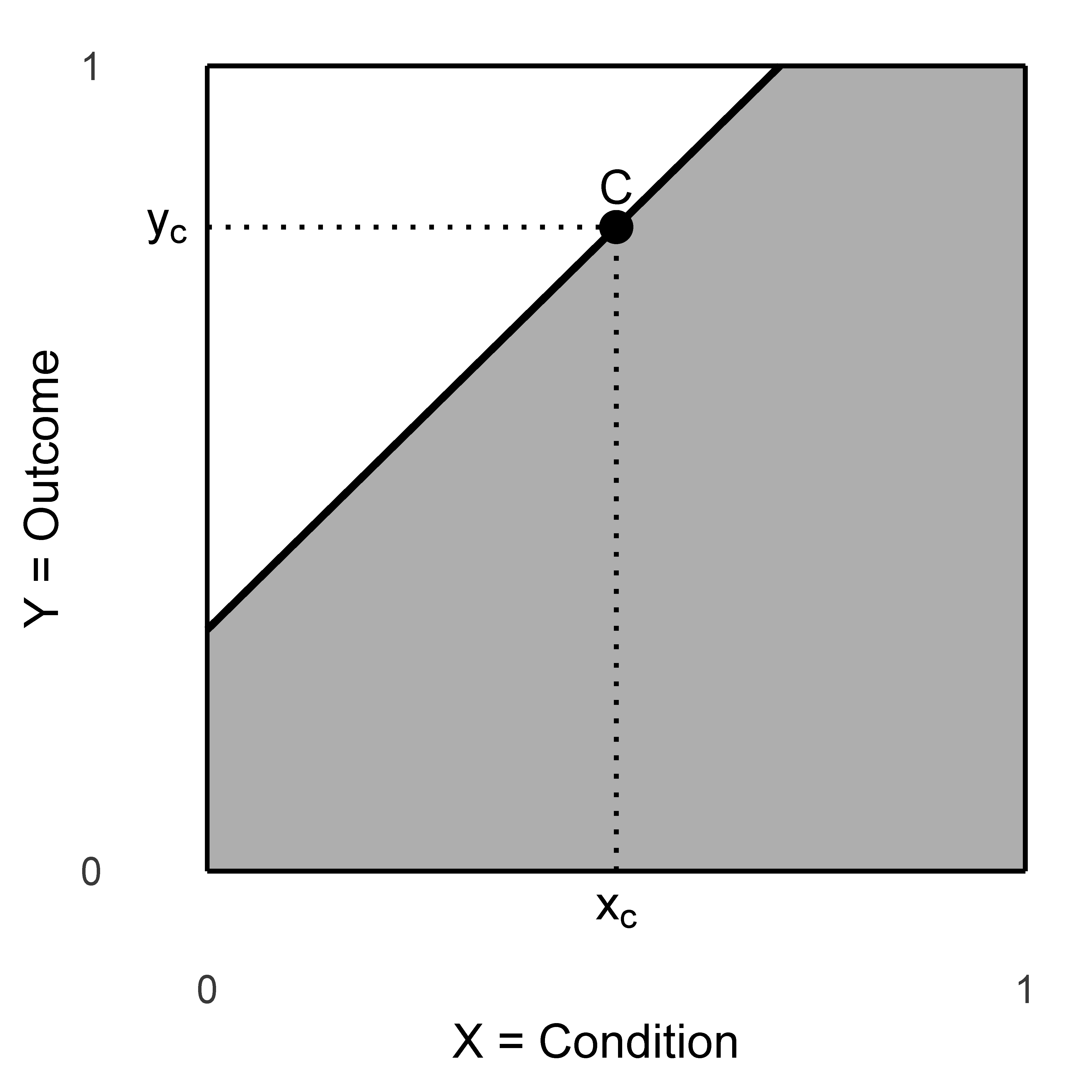
Figure 2.4: $XY$-plot illustrating necessity causality when $X$ and $Y$ are continuous (necessity-in-degree, NiD).

2.7 Causal underdetermination

A causal relationship cannot be directly observed. What can be observed are only sequences and patterns. For example, when a glass falls from the table, we see the motion of the hand, the contact with the glass, the glass’s acceleration, and its eventual impact on the ground. Nowhere in this stream of sensory data is there an observable entity called “causation.” The causal link must instead be inferred. Was the push responsible for the fall, was the table moved at the same moment, or did the glass fall by coincidence?

Because causality cannot be observed, a human interpretation of observed data must be made. The same observational data can support multiple causal explanations. This is the phenomenon known as causal underdetermination (e.g., Stanford, 2023). An observed relationship between $X$ and $Y$ may reflect that $X$ causes $Y$, $Y$ causes $X$, an unobserved cause, or mere chance. Underdetermination implies that a single dataset can be explained by different causal models, whether framed in terms of necessity, sufficiency, probabilistic tendencies, or typicality.

The idea that the same evidence can be “seen” differently is illustrated by the classic ambiguous picture below. Some viewers immediately see a young woman, while others see an old woman, and it can be hard to switch between the two. Likewise, the same data can support different causal interpretations, and once someone becomes familiar with one perspective, it may be difficult to adopt another.

$The same image can be seen in different ways. Likewise, the same data can be viewed through different causal lenses. From: My wife and my mother-in-law. They are both in this picture – find them. Prints \& Photographs Online Catalog, Library of Congress. https://www.loc.gov/pictures/item/2010652001/. Retrieved 1 October 2025.$

Figure 2.5: The same image can be seen in different ways. Likewise, the same data can be viewed through different causal lenses. From: My wife and my mother-in-law. They are both in this picture – find them. Prints & Photographs Online Catalog, Library of Congress. https://www.loc.gov/pictures/item/2010652001/. Retrieved 1 October 2025.

A related implication is the problem of non-identifiability (or observational equivalence): distinct models can generate the same observable data patterns and therefore fit the data equally well, even though they imply different underlying structures (e.g., Rothenberg, 1971). When this happens, the evidence cannot distinguish between these competing explanations. For example, when a correlation between $X$ and $Y$ is observed, this could be interpreted as a result of a probabilistic sufficiency relationship, or as a result of a necessity relationship (Appendix G). In principle, both interpretations are possible.

Given the inherent underdetermination of causal claims from observations, theory becomes indispensable. Theory provides the assumptions and background knowledge needed to justify a causal model that is consistent with the observations. Without such guiding principles, data remain compatible with infinitely many interpretations. Theory specifies, for example, which mechanisms are plausible or which temporal order is even possible. The central role of theory in data analysis for causal inference is illustrated by Nancy Cartwright’s slogan:

“No causes in, no causes out” (Cartwright, 1989, pp. 39–90)

Some causal theories may be more plausible than others. For example, if we observe that plants exposed to more sunlight grow more, the explanation that sunlight causes plant growth is far more credible than the idea that plant growth causes sunlight. An observed relationship is considered spurious when an alternative explanation is clearly more credible because the theory is more plausible or because of better model fit.¹⁹

However, several causal theories may also be equally credible. This is the situation known as causal pluralism: different causal perspectives may each illuminate different aspects of the same phenomenon (Section 11.2). Causal pluralism can help to better understand the underlying causal mechanisms of the phenomenon of interest. If several causal theories are equally credible, it is also possible to select one theory for pragmatic reasons. Such reasons could be simplicity (Section 3.3), usefulness for prediction, computational elegance, compatibility with other accepted theories, interpretability, or practical actionability. A necessity theory could be a candidate.

Underdetermination and pluralism imply that no single causal perspective is inherently the “proper” one for every study question. In particular, commonly used probabilistic sufficiency perspectives and their associated regression tools are not inherently preferred. It is the analyst’s freedom to select an appropriate perspective and tools, and the analyst’s responsibility to justify the corresponding hypothesis and interpretation (Chapter 7).

This book is about the use of the necessity causal perspective and tools when studying phenomena. It therefore follows that a necessity-based theoretical framework is essential for describing such phenomena coherently. What constitutes such a necessity theory is discussed in the next chapter.

References

Baumgartner, M. (2009). Inferring causal complexity. Sociological Methods & Research, 38(1), 71–101. https://doi-org.eur.idm.oclc.org/10.1177/0049124109339369

Campbell, J. T., & Fiss, P. C. (2026). Tackling the complexity challenge: When and how to engage in configurational and hybrid theorizing. Academy of Management Review, ja, amr–2024. https://doi.org/10.5465/amr.2024.0187

Cartwright, N. (1989). Nature’s capacities and their measurement. Clarendon Press, Oxford.

Dul, J. (2016a). Identifying single necessary conditions with NCA and fsQCA. Journal of Business Research, 69(4), 1516–1523. https://doi.org/10.1016/j.jbusres.2015.10.134

Dul, J. (2016b). Necessary Condition Analysis (NCA): Logic and methodology of “necessary but not sufficient” causality. Organizational Research Methods, 19(1), 10–52. https://doi.org/10.1177/1094428115584005

Dul, J. (2020). Conducting Necessary Condition Analysis. Sage. https://uk.sagepub.com/en-gb/eur/conducting-necessary-condition-analysis-for-business-and-management-students/book262898

Dul, J. (2024a). A different causal perspective with Necessary Condition Analysis. Journal of Business Research, 177, 114618. https://doi.org/10.1016/j.jbusres.2024.114618

Dul, J., Vis, B., & Goertz, G. (2021). Necessary Condition Analysis (NCA) does exactly what it should do when applied properly: A reply to a comment on NCA. Sociological Methods & Research, 50(2), 926–936. https://doi.org/10.1177/0049124118799383

Goertz, G., & Mahoney, J. (2012). A tale of two cultures: Qualitative and quantitative research in the social sciences. Princeton University Press. https://press.princeton.edu/books/hardcover/9780691149707/a-tale-of-two-cultures

Goldstein, S. (2012). Typicality and notions of probability in physics. Probability in Physics, 59–71. https://link.springer.com/chapter/10.1007/978-3-642-21329-8_4

Hume, D. (1756). Essays and treatises on several subjects. Volume 2, third edition. London: A. Millar.

Machamer, P., Darden, L., & Craver, C. F. (2000). Thinking about mechanisms. Philosophy of Science, 67(1), 1–25. https://www.jstor.org/stable/188611

Mackie, J. L. (1965). Causes and conditions. American Philosophical Quarterly, 2(4), 245–264. https://www.jstor.org/stable/20009173

Pearl, J. (2009). Causality. Cambridge University Press. https://www.cambridge.org/core/books/causality/B0046844FAE10CBF274D4ACBDAEB5F5B

Ragin, C. C. (1987). The comparative method: Moving beyond qualitative and quantitative strategies. JSTOR. https://www.jstor.org/stable/10.1525/j.ctt1pnx57?turn_away=true

Rothenberg, T. J. (1971). Identification in parametric models. Econometrica, 39(3), 577–591. https://doi.org/10.2307/1913267

Rothman, K. J. (1976). Causes. American Journal of Epidemiology, 104(6), 587–592. https://doi.org/10.1093/oxfordjournals.aje.a112335

Stanford, K. (2023). Underdetermination of scientific theory. In E. N. Zalta & U. Nodelman (Eds.), The stanford encyclopedia of philosophy (fall 2023 edition). Metaphysics Research Lab, Stanford University. https://plato.stanford.edu/archives/fall2023/entries/scientific-underdetermination/

Torres, P., & Godinho, P. (2022). Levels of necessity of entrepreneurial ecosystems elements. Small Business Economics, 59, 29–45. https://doi.org/10.1007/s11187-021-00515-3

Varzi, A. (2019). Mereology. In E. N. Zalta (Ed.), The stanford encyclopedia of philosophy. Edition spring 2019. https://plato.stanford.edu/archives/spr2019/entries/mereology/

Vis, B., & Dul, J. (2018). Analyzing relationships of necessity not just in kind but also in degree: Complementing fsQCA with NCA. Sociological Methods & Research, 47(4), 872–899. https://doi.org/10.1177/0049124115626179

Wagner, G. (2020). Typicality and minutis rectis laws: From physics to sociology. Journal for General Philosophy of Science, 51, 447–458. https://doi.org/10.1007/s10838-020-09505-7

Wilhelm, I. (2022). Typical: A theory of typicality and typicality explanation. The British Journal for the Philosophy of Science. https://www.journals.uchicago.edu/doi/pdf/10.1093/bjps/axz016

Wright, R. W. (1985). Causation in tort law. Calif. L. Rev., 73, 1735. https://scholarship.kentlaw.iit.edu/fac_schol/697

If $X$, then $Y$ means: if we see $X$, we also see $Y$, and if we add $X$, we get $Y$.↩︎
If not $X$, then not $Y$ means: if we do not see $X$, we also do not see $Y$, and if we remove $X$, we do not see $Y$ anymore.↩︎
Causality itself cannot be observed, see Section 2.7 and Chapter 7.↩︎
See, for example, QCA’s use of the consistency score < 1 to allow imperfect sufficiency.↩︎
Note the difference between Exception and Noise as discussed in Section 4.5.4.↩︎
Necessity-in-kind (NiK) refers to the qualitative statement that $X$ is necessary for $Y$ without specifying the level of $X$ and $Y$ other than presence/absence or low/high. This contrasts with NCA’s necessity-in-degree (NiD) where specific levels of $X$ and $Y$ are specified.↩︎
Formally, PN is defined as: $PN = P(Y_{X=0} = 0 \mid X = 1, Y = 1)$.↩︎
Until recently, I was not aware of the existence of the typicality perspective on causality. What I previously called a ‘probabilistic view’ on necessity causality (Dul, 2020) refers to what I now (Dul, 2024a) call the ‘typicality perspective’ of necessity causality (based on cardinality). The current description ‘probabilistic perspective’ of causality refers to the use of probabilities to describe causality, but this is not part of NCA.↩︎
Also in fuzzy set QCA (fsQCA) the necessary condition in the sufficiency solution is binary, see Section 11.5.↩︎
Section 6.4.2 discusses model fit in the context of NCA.↩︎