6 Credibility

6.1 Summary of this chapter

This chapter evaluates the credibility of NCA to identify necessity from data. In the context of NCA, credibility refers to the trustworthiness of conclusions about necessity from data⁶¹. The chapter starts by discussing the core criteria to draw conclusions about necessity: there must be a theoretically justified necessity hypothesis, the effect size must be practically relevant (high \(d\)-value), and the observed empty space must be unlikely to be compatible with no relationship (low \(p\)-value) (Section 6.2). A positive conclusion that necessity is supported requires that all three of these criteria are met. A negative conclusion that necessity does not exist is drawn if any of the three is not satisfied. Next, the chapter evaluates the statistical credibility of NCA using Monte Carlo simulations to analyze how well NCA detects necessity when it is present in the population (True Positive Rate-TPR, sensitivity) and how well NCA avoids detecting necessity when it is absent in the population (True Negative Rate-TNR, specificity) (Section 6.3). Subsequently, the empirical credibility of an NCA study is evaluated focusing on robustness checks (the extent to which the findings are not dependent on the analyst’s choices) and model fit metrics (the extent to which the necessity model matches the data) (Section 6.4). Finally, recommendations are given on how to evaluate the credibility of a specific study (Section 6.5).

6.2 Core criteria for necessity

NCA draws a positive conclusion about necessity if three requirements are jointly satisfied: there is theoretical support for necessity (a formal necessity hypothesis), there is a reasonably large effect size (e.g., \(d \geq 0.10\)), and there is a reasonably small \(p\)-value (e.g., \(p < 0.05\)). NCA draws a negative conclusion about necessity if one or more of these requirements are not met.

To meet the requirement of theoretical support, the analyst formulates and theoretically justifies that \(X\) and \(Y\) are causally related by necessity as outlined in Chapter 7. One implication is that the analyst expects emptiness of a specific corner in the \(XY\)-plot. For example, if it is expected that a high level of \(X\) is necessary for a high level of \(Y\), no high values of \(Y\) are expected when \(X\) is low. Therefore, the upper-left corner of the \(XY\)-plot is expected to be empty. If no theoretical support for necessity is provided, NCA draws a negative conclusion about necessity, even if effect size and \(p\)-value satisfy the criteria.

To meet the requirement of a minimum effect size, NCA estimates the size of the empty space in the expected empty corner of the sample’s \(XY\)-plot (\(d\)-value) and judges whether this size is relevant by comparing it with the selected threshold \(d\)-value (e.g., \(d \geq 0.10\)). If this requirement for a relevant \(d\)-value is not met, NCA draws a negative conclusion about necessity even if there is theoretical support and the \(p\)-value is below the threshold \(p\)-value.

To meet the requirement of a maximum \(p\)-value, NCA’s statistical test is conducted to estimate the \(p\)-value of the estimated necessity effect size, and a comparison is made with the selected threshold \(p\)-value (e.g., \(\alpha = 0.05\)). One unique feature of this test is that it uses the size of the expected empty space as the test statistic, thus testing the randomness of this specific emptiness when \(X\) and \(Y\) are unrelated, rather than being a general randomness test (Section 5.3). If the requirement for a small \(p\)-value (e.g., \(p < 0.05\)) is not met, NCA draws a negative conclusion about necessity.⁶²

Only if all requirements are met, NCA draws a positive conclusion about necessity in the population (within the common limitations of a study design, and acknowledging the need for replications). If one of them is not met, NCA draws a negative conclusion about necessity in the population. This set of requirements for drawing a conclusion about necessity in the population shows that NCA is more than just a statistical model and that evaluating necessity with just the \(p\)-values is not enough. NCA’s statistical test and \(p\)-value are only one part of the process of making a conclusion about necessity. This fits the commonly accepted view that conclusions about empirically observed effects should not be solely based on the \(p\)-value, but also on effect size and theoretical argumentation (see for instance, Cohen, 1994; Cumming, 2013; Greenland & Robins, 1986; Rothman & Greenland, 2005; Wasserstein & Lazar, 2016). Although isolated statistical null hypothesis tests are usually evaluated with concepts like type I error, type II error and power, these concepts are not enough for evaluating the credibility of the NCA approach as a whole, where other non-statistical criteria are also relevant (theoretical support, effect size).

6.3 Statistical credibility

To evaluate the credibility of a binary classification like NCA’s positive or negative conclusion about necessity in the population, the True Positive Rate (TPR or sensitivity) and True Negative Rate (TNR or specificity) can be used. Applied to NCA, TPR is the ability of the approach to correctly identify that necessity exists in a population, and TNR is the ability of the approach to correctly identify that necessity is absent in a population. ‘Rate’ refers to the proportion of randomly drawn samples from that population that were correctly evaluated regarding the presence or absence of necessity.

For testing the credibility of NCA with these evaluation criteria, a Monte Carlo simulation is performed. The simulation evaluates TPR and TNR based on the analysis of samples from two populations: one with the necessary condition (for evaluating TPR), and one without it (for evaluating TNR), and using the three criteria to identify necessity. The simulation assumes that the requirement of ‘theoretical support’ is satisfied. This implies that it is clear which corner of the sample \(XY\)-plot is the expected empty corner and must be analyzed. Here the theoretical expectation is that a high value of \(X\) is necessary for a high value of \(Y\), resulting in the upper-left corner as the expected empty corner (corner 1; Section 3.6). As a reminder, the numbering of the corners is shown in Figure 6.1.

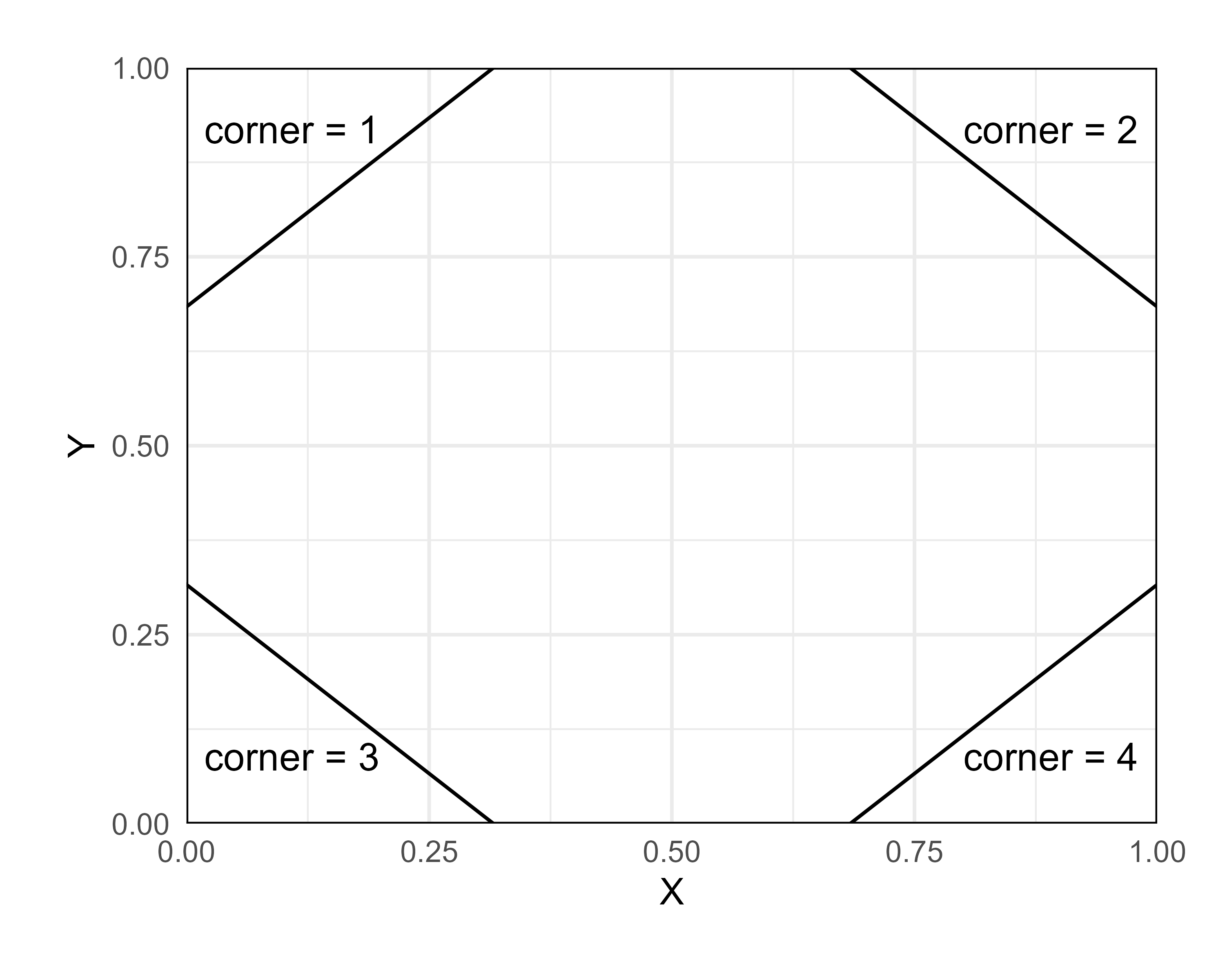
Figure 6.1: Numbering of corners in an \(XY\)-plot.

For testing the TPR, the simulation must ensure that necessity is present in the upper-left corner of the population \(XY\)-plot, so that this corner is empty. Since for testing TPR all samples are drawn from a population where necessity is always present (rather than being present with a certain probability), the False Negative Rate (FNR) equals 1 − TPR. Similarly, for testing TNR, the simulation must ensure that necessity is absent in the upper-left corner in the population \(XY\)-plot, thus that this corner is not empty. Since for testing TNR all samples are drawn from a population where necessity is not present, the False Positive Rate (FPR) equals 1 − TNR. Together with the True Positive Rate (TPR), these two measures reflect the model’s ability to correctly classify both presence and absence of necessity.

For both tests (TPR and TNR) four scenarios are simulated. In scenario A, \(X\) and \(Y\) are only related by necessity in the expected empty corner (for testing TPR), or are not related by necessity in the expected empty corner (for testing TNR). In this scenario no other relationships exist between \(X\) and \(Y\). In the other scenarios (scenarios B, C, and D) it is assumed that other relationships exist as well. Although an infinite number of types of relationships (bivariate distributions) could exist, here the focus is on other necessity relationships than the one in the upper-left corner. The other relationships produce emptiness in other corners than the corner of interest. However, none of the other relationships are hypothesized or tested. The only goal of additional empty corners in the simulation is to challenge NCA’s credibility regarding necessity related to the hypothesized empty corner, when other relationships are also present. The four simulation scenarios about necessity and other relationships in the population are therefore:

A. Necessity (TPR) or non-necessity (TNR) in corner 1. No other relationships.

B. Necessity (TPR) or non-necessity (TNR) in corner 1. Other relationship in corner 2.

C. Necessity (TPR) or non-necessity (TNR) in corner 1. Other relationship in corner 3.

D. Necessity (TPR) or non-necessity (TNR) in corner 1. Other relationship in corner 4.

In all scenarios \(X\) and \(Y\) are related (TPR) or unrelated (TNR) by necessity in the upper-left corner. In scenario A there is no other relationship. In the other scenarios \(X\) and \(Y\) are (also) otherwise related because one of the other corners than the expected empty corner of interest is empty⁶³.

The technical details of the Monte Carlo simulation are as follows. Since NCA requires bounded variables, the bounding box (Section 4.3.1) in the population where cases could exist is defined by the unit box in which \(X\)- and \(Y\)-values can range from 0 to 1 (scope = 1). The true feasible area of the population (within the bounding box) is the entire unit box when \(X\) and \(Y\) are unrelated and is a part of the unit box when \(X\) and \(Y\) have the necessity relationship. The empty corner is assumed to be a triangle consisting of the area between a linear ceiling line (corners 1 and 2) or a linear floor line (corners 3 and 4) and the borders of the unit box. The slopes of the ceiling and floor lines are 1 for corners 1 and 4 and \(-1\) for corners 2 and 3. The sizes of the empty corner range from 0 to a maximum of 0.50. The combination of slope and empty area determines the intercepts of the lines as follows:

corner 1: \(a_1 = 1 - \sqrt{2e_1 b_1}\).

corner 2: \(a_2 = 1 + |b_2| - \sqrt{2e_2 |b_2|}\).

corner 3: \(a_3 = \sqrt{2e_3 |b_3|}\).

corner 4: \(a_4 = 0 - (b_4 - \sqrt{2e_4 b_4})\).

where \(a\) is the intercept and \(b\) is the slope of the line, and \(e\) is the size of the empty space. The subscripts indicate the corresponding corner. For the expected empty corner, the size of the empty space equals the necessity effect size (\(d\)) since the scope equals 1. When two opposite corners are empty, the two lines are parallel and when two adjacent corners are empty, the two lines intersect. In the latter situation it is possible that for larger necessity effect sizes and empty space sizes the two lines intersect within the bounding box (Figure 6.2). This reduces the intended necessity effect size, empty space size and scope. In the simulation this situation is avoided to keep the results comparable. Consequently, higher sizes of adjacent empty corners are not evaluated.

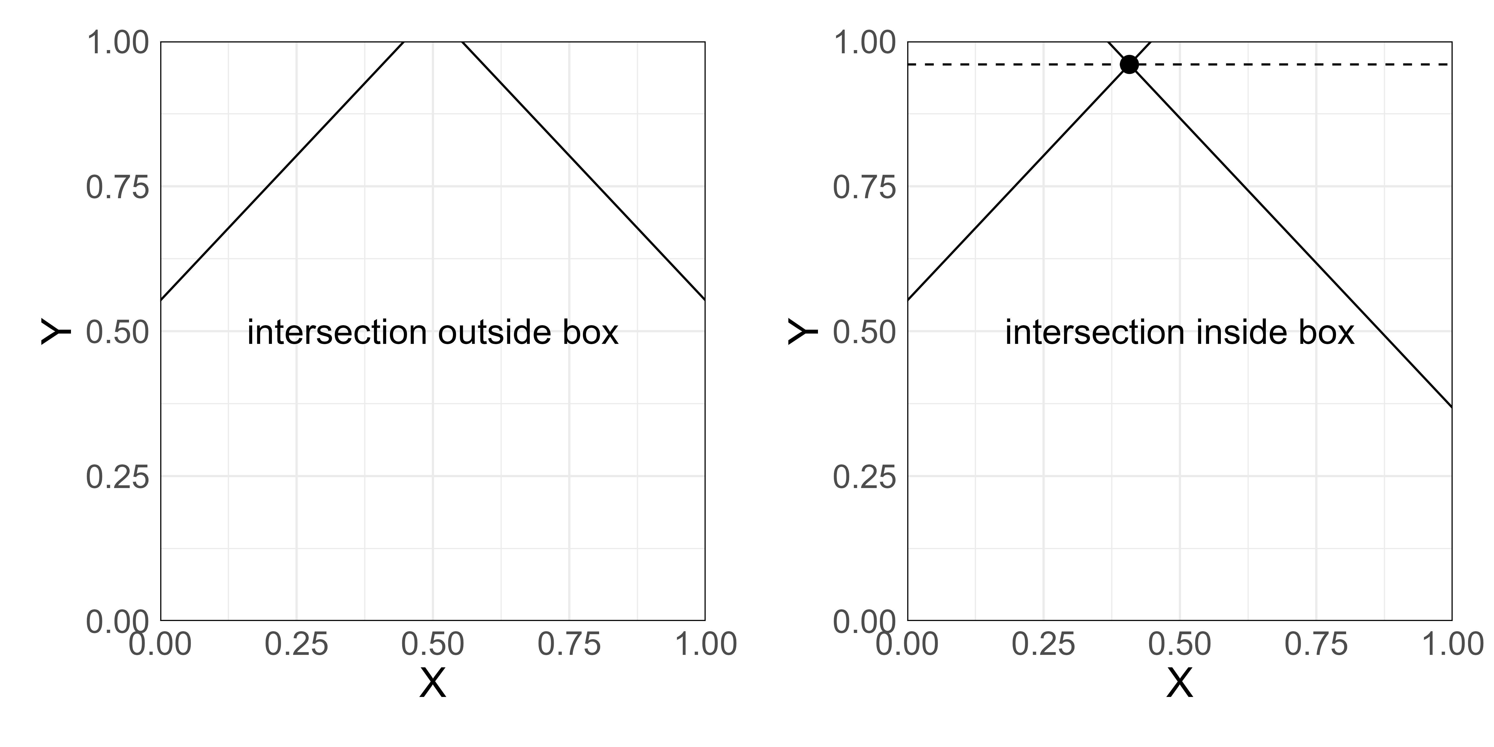
Figure 6.2: Intersection of two adjacent empty corners. Left: The lines intersect outside the bounding box. Necessity effect size of corner 1 is 0.1. Size of empty corner 2 is 0.1. Scope = 1. Right: The lines intersect inside the bounding box. Intended necessity effect size is 0.1. Reduced necessity effect size is < 0.1. Intended size of empty corner 2 is 0.2. Reduced size of empty corner 2 is < 0.2. Reduced scope < 1.

It is assumed that within the non-empty area of the bounding box the cases have a uniform distribution (Section 5.4). The nca_random function of the NCA software in R is used to create such a distribution in the presence of a ceiling line. From this defined population, 1000 random samples are drawn. Subsequently, for each sample the size of the expected empty corner (necessity effect size) is estimated with the CE-FDH ceiling line (with empirical scope). The \(p\)-value for each sample is estimated using 1000 random samples from the permutation distribution. The threshold \(p\)-value is set at 0.05. This means that necessity is considered not supported (negative conclusion) if the \(p\)-value is 0.05 or larger. If the \(p\)-value is below 0.05, necessity is considered supported (positive conclusion) only if the other two criteria (theoretical support and effect size) are also met. The theoretical support is assumed to be met. For the effect size the threshold \(d\)-value is 0.10. If applicable and possible, the tested sizes of the other empty corner are 0.05, 0.10, 0.20, 0.30, and 0.50.

6.3.1 True Positive Rate (TPR, sensitivity)

Figure 6.3 shows the results of the evaluation of TPR for a true necessity effect size of \(d\) = 0.10 in corner 1, the expected empty corner (called necessity corner in the figure), and with different sizes of other empty corner 2 (Figure 6.3-top-right), other empty corner 3 (Figure 6.3-bottom-left) and other empty corner 4 (Figure 6.3-bottom-right).

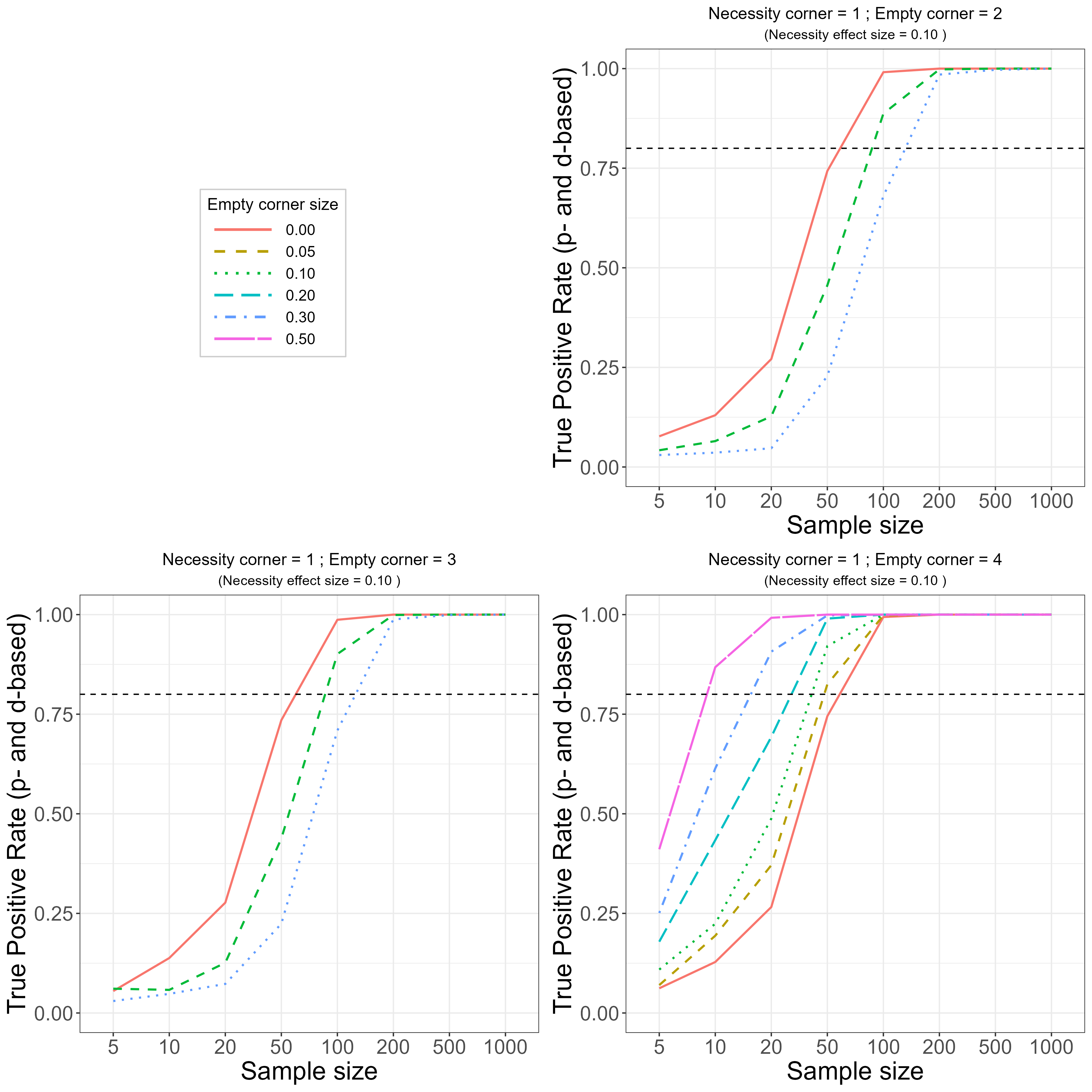
Figure 6.3: True Positive Rate (TPR, sensitivity) of the NCA approach for identifying necessity in the population. True necessity effect size in corner 1 = 0.10. Slopes of ceiling/floor lines are 1 (corners 1 and 4) or \(-1\) (corners 2 and 3). Top-Right: other empty corner = 2. Bottom-Left: other empty corner = 3. Bottom-Right: other empty corner = 4.

In all three graphs, the necessity effect size (the size of the expected empty corner 1) is 0.10, and the size of another empty corner ranges from 0 to 0.50, where possible. A TPR value of 0.80 is added as a benchmark, meaning that for 80 percent of the samples a correct decision is made, namely concluding that necessity is present in the population. This selected value is inspired by the commonly used target of 0.80 for statistical power. NCA draws a positive conclusion about necessity if \(p < 0.05\) and \(d\geq 0.10\) (assuming theoretical support).

Scenario A applies when the other corners are not empty. The corresponding TPR curve is the same in each TPR graph (empty corner size = 0). This curve is the upper curve in the Top-Right and Bottom-Left graphs, and the lower curve in the Bottom-Right graph. In scenario A, TPR increases with sample size and the benchmark value of 0.80 (80% correct decisions when necessity is present in the population) is reached for a sample size of about 60 (note that the horizontal axis is piecewise-linear: linear between two adjacent ticks but not across ticks).

Table 6.1-top-left shows for scenario A the fraction of samples where \(p < 0.05\) (\(p\)-based TPR) and the fraction of samples where \(d \geq 0.10\) (\(d\)-based TPR). Considering both criteria, TPR is the minimum of \(p\)-based TPR and \(d\)-based TPR. It turns out that for scenario A, the \(p\)-value criterion (\(p < 0.05\)) is critical for the TPR conclusion. Consequently, TPR corresponds to the power of NCA’s statistical test in this simulation scenario.

Table 6.1: Fraction of samples that correctly identify necessity: p-based, d-based, TPR (True Positive Rate). Necessity effect size = 0.10 (corner 1 empty) with ceiling slope = 1. Top-Left table: Scenario A – no other corner empty. Top-Right table: Scenario B – corner 2 also empty. Bottom-Left table: Scenario C – corner 3 also empty. Bottom-Right table: Scenario D – corner 4 also empty. Other empty corner size = 0.10.

n p-based d-based TPR 5 0.077 0.801 0.077 10 0.130 0.890 0.130 20 0.271 0.971 0.271 50 0.743 0.995 0.743 100 0.991 0.999 0.991 200 1.000 1.000 1.000 500 1.000 1.000 1.000 1000 1.000 1.000 1.000	n p-based d-based TPR 5 0.030 0.715 0.030 10 0.036 0.815 0.036 20 0.047 0.895 0.047 50 0.228 0.954 0.228 100 0.680 0.980 0.680 200 0.985 0.993 0.985 500 1.000 0.997 0.997 1000 1.000 1.000 1.000
n p-based d-based TPR 5 0.030 0.725 0.030 10 0.048 0.815 0.048 20 0.073 0.889 0.073 50 0.224 0.946 0.224 100 0.709 0.978 0.709 200 0.988 0.994 0.988 500 1.000 0.999 0.999 1000 1.000 1.000 1.000	n p-based d-based TPR 5 0.109 0.843 0.109 10 0.224 0.936 0.224 20 0.488 0.979 0.488 50 0.921 0.995 0.921 100 1.000 1.000 1.000 200 1.000 1.000 1.000 500 1.000 1.000 1.000 1000 1.000 1.000 1.000

Scenario B applies when corner 2 (upper-right corner) is also empty (empty corner size = 0.05 or 0.10, see Figure 6.3-top-right). It turns out that the TPR curve shifts to the right with increasing emptiness of corner 2, meaning that for a given sample size the TPR decreases when the emptiness of corner 2 increases. Consequently, higher sample sizes are required to be able to identify necessity in corner 1 if this exists in the population. When the emptiness of corner 2 increases, relatively fewer cases are available to statistically test the emptiness of corner 1. NCA’s statistical test uses a permutation procedure (Section 5.3) that creates new cases by allocating \(Y\)-values of observed cases randomly to \(X\)-values of other observed cases, and random samples are drawn from the obtained permutation distribution (= null distribution). High \(Y\)-values of cases allocated to low \(X\)-values of other cases can challenge the emptiness of corner 1. If relatively fewer high \(Y\)-values are available, the sample size must be larger to have enough high \(Y\)-values for the test. For achieving a TPR of 0.80, the required sample size is about 75 if the size of the empty corner 2 is 0.05 and about 140 if this size is 0.10.

Table 6.1-top-right shows that also in scenario B the \(p\)-value criterion (\(p < 0.05\)) and not the \(d\)-value criterion (\(d \geq 0.10\)) is critical for the TPR conclusion (with one exception for n = 500 where the \(d\)-based TPR is smaller than the \(p\)-based TPR).

Scenario C (Figure 6.3-bottom-left) applies when corner 3 (lower-left corner) is also empty (empty corner size = 0.05 or 0.10). The graph is very similar to that of scenario B, with some minor differences at lower values of sample size. Also in this scenario higher sample sizes are required to be able to identify necessity in corner 1 when corner 3 is more empty. For achieving a TPR of 0.80, the required sample size is also about 75 if the size of the empty corner 3 is 0.05 and about 140 if this size is 0.10.

Also in scenario C the \(p\)-value criterion (\(p < 0.05\)) is dominant.

However, in scenario D the results are very different (Figure 6.3-bottom-right). In this scenario, corner 4 (lower-right corner) is also empty (empty corner size ranges from 0.05 to 0.50). Now the TPR curve shifts to the left with increasing emptiness of corner 4, meaning that for a given sample size the TPR credibility of the NCA approach increases. This means that smaller sample sizes can be used to identify necessity in corner 1. When corner 4 is empty (and corners 2 and 3 are not empty) relatively more cases are available to test the emptiness of corner 1 such that the sample size can be smaller for the permutation test. For achieving a TPR of 0.80 the required sample size can be less than 50 when the corner size is 0.05 and even less than 10 when the corner 4 size is 0.50. However, the possibility of using relatively small sample sizes for identifying necessity has a price in terms of TNR (see below). Also in scenario D the \(p\)-value criterion (\(p < 0.05\)) is critical for the conclusion about TPR (Table 6.1-bottom-right).

Additional TPR simulations with a different necessity effect size (0.20), and different ceiling slopes (0.6, 1.67) in the expected empty corner can be found in Appendix E. These simulations show similar TPR patterns.

6.3.2 True Negative Rate (TNR, specificity)

Figure 6.4 shows the results of the evaluation of TNR.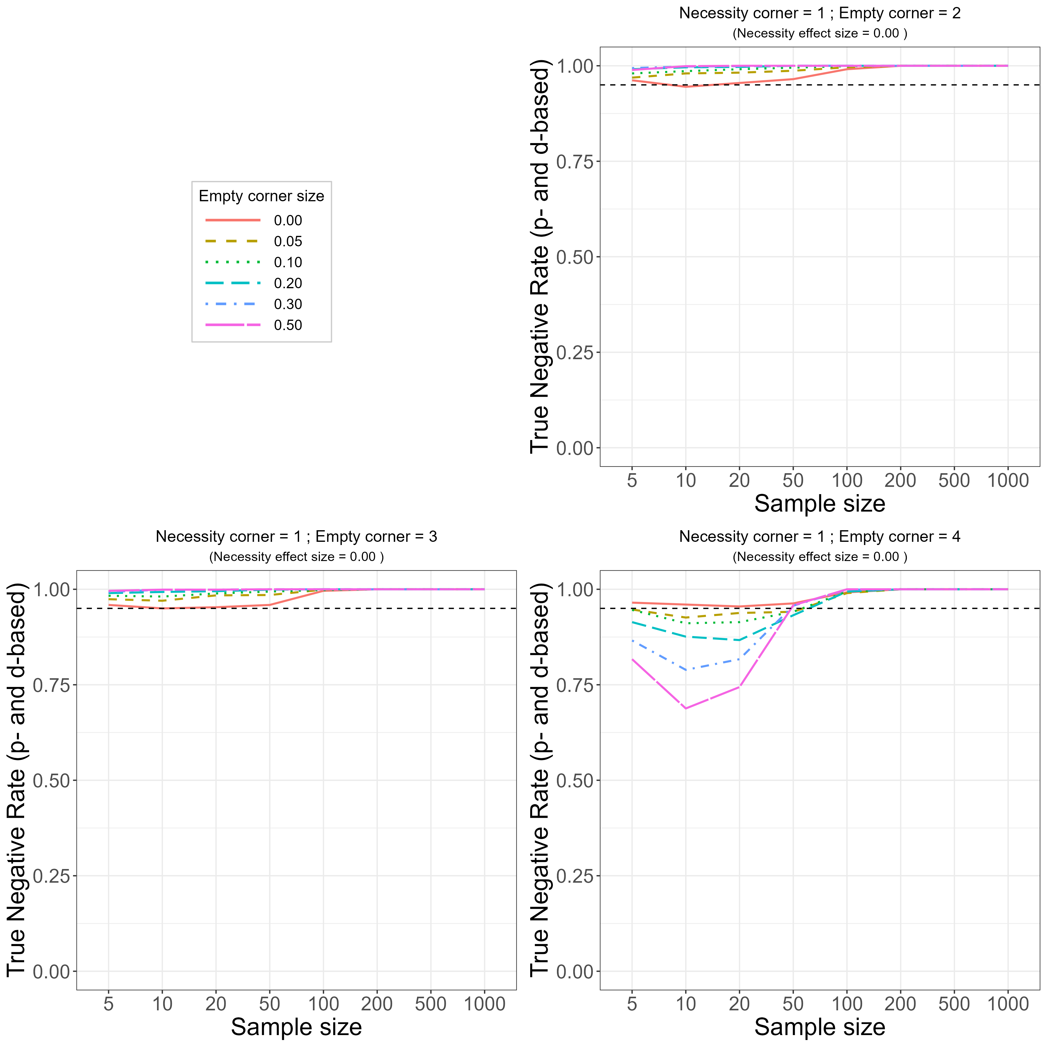

Figure 6.4: True Negative Rate (TNR, specificity) of the NCA approach for identifying non-necessity in the population. True necessity effect size in corner 1 = 0 for different sizes of other empty corners. Top-Right: other empty corner = 2. Bottom-Left: other empty corner = 3. Bottom-Right: other empty corner = 4.

In all three graphs (Top-Right, Bottom-Left, Bottom-Right) the expected empty corner is not empty (necessity effect size = 0), while the other corners are empty with sizes ranging from 0 to 0.50. A TNR value of 0.95 is added as a benchmark, meaning that the rate of correct decisions confirming the absence of necessity in the population is 0.95. This selected value is inspired by the commonly selected threshold \(p\)-value of 0.05 for the false positive rate of a statistical test. NCA draws a negative conclusion about necessity if \(p \ge 0.05\) or \(d < 0.10\).

In the TNR evaluation, scenario A applies when not only the expected corner is not empty (necessity effect size = 0) but also the other corners are not empty (empty corner size = 0), such that no relationship exists in the population. The corresponding TNR curves in Figure 6.4 are the same, which are the lowest curves for the Top-Right and Bottom-Left graphs and the highest curve for the Bottom-Right graph. The curve shows that for all sample sizes the TNR is at least 0.95. Up to a sample size of 50, TNR is constant at 0.95 and when the sample size increases the TNR curve moves upward toward 1. The reason is that as long as the \(p\)-value is critical, 1 − TNR = FNR corresponds to the \(p\)-value of NCA’s statistical test: 5% of the samples drawn from a population where \(X\) and \(Y\) are unrelated (corresponding to scenario A in the TNR test) are false positives, and 95% are true negatives.

Table 6.2: Fraction of samples that correctly identify the absence of necessity: p-based, d-based, TNR (True Negative Rate). Corner 1 is tested for necessity (corner 1 not empty). Top-Left table: Scenario A – no other corner empty. Top-Right table: Scenario B – corner 2 empty. Bottom-Left table: Scenario C – corner 3 empty. Bottom-Right table: Scenario D – corner 4 empty. Other empty corner size = 0.10.

n p-based d-based TNR 5 0.962 0.413 0.962 10 0.945 0.430 0.945 20 0.954 0.598 0.954 50 0.954 0.877 0.954 100 0.953 0.988 0.988 200 0.942 1.000 1.000 500 0.952 1.000 1.000 1000 0.950 1.000 1.000	n p-based d-based TNR 5 0.980 0.515 0.980 10 0.986 0.577 0.986 20 0.991 0.705 0.991 50 0.994 0.944 0.994 100 0.997 0.998 0.998 200 0.997 1.000 1.000 500 0.999 1.000 1.000 1000 0.997 1.000 1.000
n p-based d-based TNR 5 0.983 0.479 0.983 10 0.981 0.539 0.981 20 0.989 0.718 0.989 50 0.992 0.935 0.992 100 0.993 0.994 0.994 200 0.998 1.000 1.000 500 1.000 1.000 1.000 1000 0.999 1.000 1.000	n p-based d-based TNR 5 0.946 0.371 0.946 10 0.910 0.408 0.910 20 0.913 0.596 0.913 50 0.917 0.890 0.917 100 0.905 0.992 0.992 200 0.910 1.000 1.000 500 0.896 1.000 1.000 1000 0.918 1.000 1.000

Table 6.2 shows the fraction of samples where \(p \ge 0.05\) (\(p\)-based TNR) and the fraction of samples where \(d < 0.10\) (\(d\)-based TNR).

Since for each sample NCA draws a negative conclusion about necessity if \(p \geq 0.05\) or \(d \leq 0.10\), TNR is the maximum of \(p\)-based TNR and \(d\)-based TNR.

Table 6.2-top-left for scenario A indicates that up to sample size 50 the \(p\)-value TNR dominates and when the sample size increases, the TNR is based on the \(d\)-value. In other words, nearly all samples are correctly evaluated when necessity is absent in the population and other corners are not empty.

Scenario B for TNR (Figure 6.4-top-right) applies when necessity is absent while corner 2 (upper-right corner) is empty (empty corner effect size = 0.05 to 0.50). It turns out that the TNR curves are above the 0.95 benchmark for all sample sizes. Nearly all samples are correctly evaluated when necessity is absent in the population and corner 2 is empty.

Table 6.2 top-right shows that for smaller sample sizes the \(p\)-value TNR is dominant, whereas for larger sample sizes the \(d\)-value TNR dominates, although the differences are small.

The situation for scenario C for TNR (Figure 6.4-bottom-left) when necessity is absent while corner 3 is empty (empty corner effect size = 0.05 to 0.50) is very similar to scenario B. In this scenario, nearly all samples are correctly evaluated when necessity is absent in the population and corner 3 is empty, and the \(p\)-value is the primary limiting factor for TNR (Table 6.2-bottom-left).

In scenario D for TNR (Figure 6.4-bottom-right), necessity is absent while corner 4 is empty (empty corner effect size ranges from 0.05 to 0.50). The results are now very different. The TNR curves start below the 0.95 benchmark and with increasing sample size move first downward and then upward and end up above the 0.95 benchmark while moving toward 1. This means that only for a sample size of more than about 50, nearly all samples are correctly evaluated. The pattern of the TNR curve can be explained by the fact that first the \(p\)-value is the limiting factor, and subsequently the \(d\)-value (Table 6.2-bottom-right).

Similar patterns of the TNR curves can be observed when the distribution in the feasible space is based on a normal rather than uniform distribution of the cases (Appendix E).

If the \(d\)-value were not included as decision criterion for necessity, TNR would have been considerably lower for scenario D. This is shown in Figure 6.5 where the TNR decision is only based on the \(p\)-value. Figure 6.5-bottom-right shows that TNR decreases with increasing sample size and increasing size of empty corner 4.⁶⁴

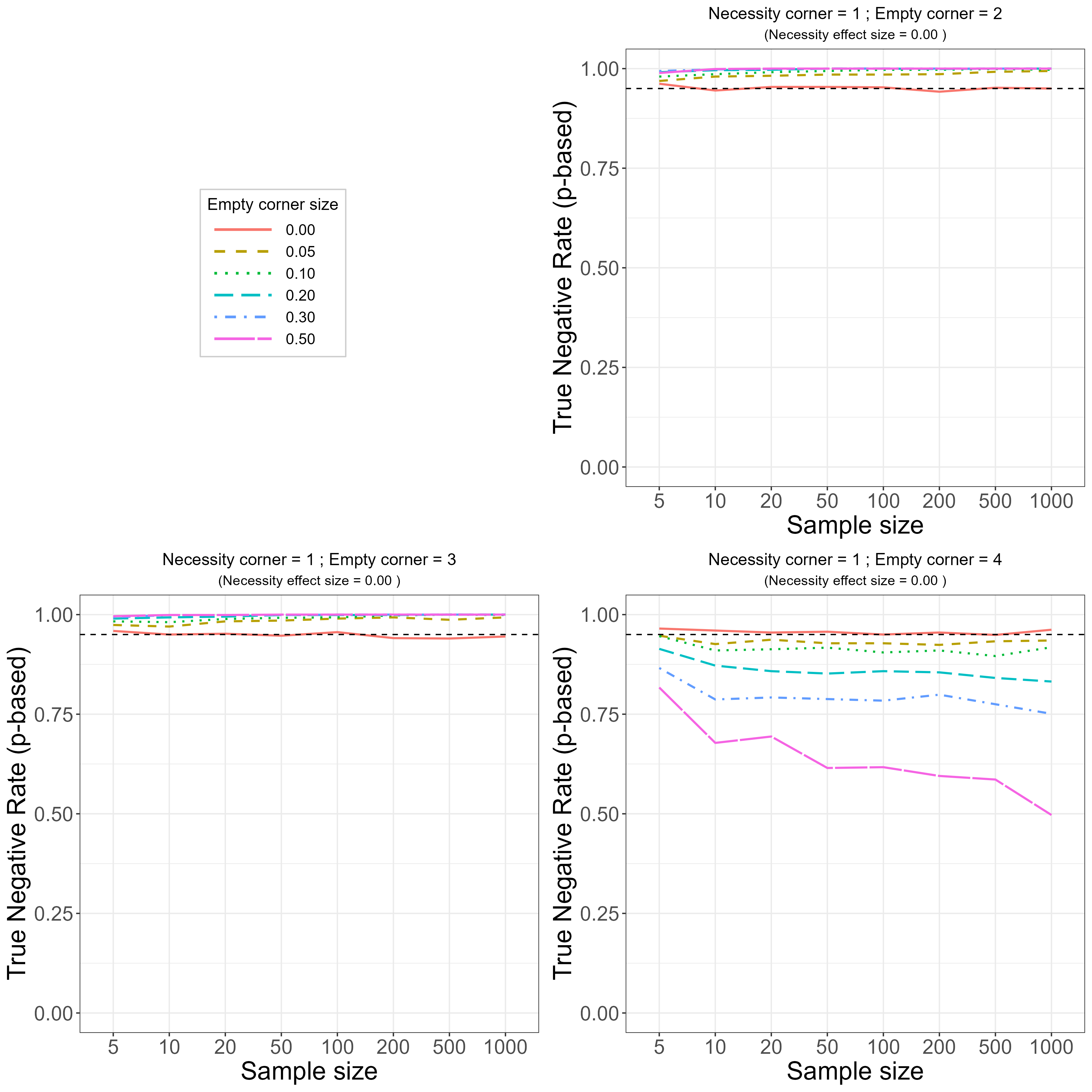
Figure 6.5: True Negative Rate (TNR, specificity) of the NCA approach for identifying necessity in the population with only the \(p\)-value criterion. True necessity effect size in corner 1 = 0 for different other empty corner sizes. Top-Right: empty corner = 2. Bottom-Left: empty corner = 3. Bottom-Right: empty corner = 4.

Because NCA bases its judgement about necessity not only on the \(p\)-value but also on the \(d\)-value (and on the availability of theoretical support), the methodology has credibility regarding both TPR and TNR, and the analyst is reasonably protected against making both false positive and false negative conclusions.

6.4 Empirical credibility

The previous results show that it is possible to identify necessary conditions when they exist, and to correctly determine when they do not exist. Nevertheless, even when the criteria for necessity (theoretical support, large \(d\)-value, low \(p\)-value) are satisfied, the TPR and TNR results also show that there is still a possibility that necessary conditions are not identified when they exist, or that they are identified when they do not exist. This can also happen when limitations exist regarding the quality of model specification (Section 4.3), study design, sampling, and measurement (Chapter 8), or data analysis (Chapter 9). To further evaluate the credibility of an NCA finding, several empirical credibility approaches may be considered.

6.4.1 Robustness

When conducting an empirical study, the analyst must make various theoretical and methodological choices to obtain results. Often, other plausible choices could also have been made. In a robustness check, the sensitivity of the results to other plausible choices is evaluated. The check focuses on the sensitivity of the main estimates and the analyst’s main conclusion.

In NCA, the effect size and the \(p\)-value are two main estimates for concluding whether a necessity relationship is credible. These estimates can be sensitive to several choices. Some choices are outside the realm of NCA, for example choices related to the data that are used as input to NCA (see Chapter 8 about study design, sampling, and measurement) or the threshold level of statistical significance. Other choices are NCA-specific, such as the choice of the ceiling line (Section 4.3.2) and the bounding box (Section 4.3), the threshold level of the necessity effect size (Section 4.4.1), and the handling of NCA-relevant outliers (Section 9.8). The credibility of support for necessity increases when the results are robust. Section 9.12 provides further details of NCA’s robustness checks.

6.4.2 Model fit

Section 4.5 introduced eight model fit metrics: complexity, fit, ceiling accuracy, noise, exceptions, support, spread, and sharpness. The credibility of the evidence for necessity increases when the model better fits the data.

6.5 Recommendations for evaluating credibility

The three core criteria for establishing necessity (theoretical support, practical relevance in terms of large effect size, and statistical relevance in terms of small \(p\)-value), the robustness check requirement, and the eight model-fit metrics are summarized in Table 6.3. The table provides examples of numerical guidelines, but these should not be interpreted as strict decision rules. Ultimately, credibility is a matter of informed judgment and optimization by the analyst and other stakeholders after considering all credibility aspects. In an empirical study, it is rare for all credibility aspects to be fully satisfied.

Table 6.3: Credibility aspects of NCA

Credibility aspect	Goal	Description	Symbol	Guideline
Theoretical support	Identifies expected empty corner. Allows interpretation of findings.	Necessity hypothesis.	H1	Specify formal necessity hypothesis.
Practical relevance	Ensures relevance of findings.	Effect size.	\(d\)	High (e.g., \(d\) \(\geq\) 0.10).
Statistical significance	Tests whether the observed effect could arise by chance (permutation test).	\(p\)-value.	\(p\)	Low (e.g., \(p\) < 0.05).
Robustness	Checks sensitivity of findings.	Repeated analysis.	\(\Delta\)\(d\), \(\Delta\)\(p\)	Report.
Model fit – complexity	Quantifies model complexity used to balance parsimony against accuracy.	Half of ceiling degrees of freedom.	\(cp\)	Balance.
Model fit – fit	Quantifies how close the chosen ceiling line is to the standard ceiling line (CE-FDH).	Alignment with boundary pattern (% effect size compared to CE-FDH effect size).	\(ft\)	High (e.g., \(ft\) \(\geq\) 80%).
Model fit – ceiling accuracy	Quantifies the degree to which the expected empty corner is indeed empty.	Percentage of points in the feasible area.	\(ca\)	High (e.g., \(ca\) \(\geq\) 95%).
Model fit – noise	Quantifies uncertainty around the ceiling line due to minor deviations.	Percentage of points in the ceiling zone near the ceiling (medP-zone).	\(ns\)	Low (e.g., \(ns\) \(\leq\) 5%; 0.9 iso-purity).
Model fit – exceptions	Quantifies violations in the ceiling zone far from the ceiling line, indicating how strict (or tolerant) the necessity claim is.	Number of points in the ceiling zone far from the ceiling (lowP-zone).	\(ex\)	Very low (e.g., \(ex\) ~0).
Model fit – support	Quantifies how strongly the data in the feasible area support the ceiling line.	Percentage of points in the feasible area on or near the ceiling (medS-zone).	\(su\)	High (e.g., \(su\) \(\geq\) 5%; 0.8 iso-solidity).
Model fit – spread	Quantifies the extent to which observations in the feasible area near the ceiling are dispersed, rather than clustered along the ceiling line.	Evenness of \(x\)-positions of points on or near the ceiling (medS-zone).	\(sp\)	High (e.g., \(sp\) \(\geq\) 0.5).
Model fit – sharpness	Quantifies how abrupt the transition in the data is across the boundary between ceiling zone and feasible area.	Relative density of points in medium-purity (medP) and medium-solidity (medS) zones.	\(sh\)	High (e.g., \(sh\) > 0.8).

In the following Part II of the book, the principles of NCA as discussed in Part I are applied to empirical studies.

References

Cohen, J. (1994). The earth is round (p<. 05). American Psychologist, 49(12), 997. https://doi.org/10.1037/0003-066X.49.12.997

Cumming, G. (2013). Understanding the new statistics: Effect sizes, confidence intervals, and meta-analysis. Routledge. https://www.taylorfrancis.com/books/mono/10.4324/9780203807002/understanding-new-statistics-geoff-cumming

Dul, J., Van der Laan, E., & Kuik, R. (2020). A statistical significance test for Necessary Condition Analysis. Organizational Research Methods, 23(2), 385–395. https://doi.org/10.1177/1094428118795272

Greenland, S., & Robins, J. M. (1986). Identifiability, exchangeability, and epidemiological confounding. International Journal of Epidemiology, 15(3), 413–419. https://doi.org/10.1093/ije/15.3.413

Rothman, K. J., & Greenland, S. (2005). Causation and causal inference in epidemiology. American Journal of Public Health, 95(S1), S144–S150. https://doi.org/10.2105/AJPH.2004.059204

Wasserstein, R. L., & Lazar, N. A. (2016). The ASA statement on p-values: Context, process, and purpose. The American Statistician, 70(2), 129–133. https://doi.org/10.1080/00031305.2016.1154108

---

61. Credibility in NCA is conceptually unrelated to the same term as used in Bayesian statistics, where it denotes probabilistic confidence in parameter estimates.↩︎

62. This requirement does not apply in a small-n study with purposeful rather than random selection of cases.↩︎

63. The results remain the same if the simulations are done with a different expected empty corner and corresponding other corners.↩︎

64. All simulations show again that when scenario A applies in Figures 6.4 and E.4 with the curves for other corner size = 0 and in Table 6.2-top-left, and when the \(p\)-value is dominant, NCA’s statistical test is valid (Dul, Van der Laan, et al., 2020).↩︎