8 Data

8.1 Summary of this chapter

This chapter describes the steps between the hypothesis and data analysis that are needed to obtain empirical data for testing a formal necessity hypothesis. The hypothesis discussed in the previous chapter (Chapter 7) guides which data should be collected. The hypothesis has precise definitions of (1) the focal unit, (2) the concepts \(X\) and \(Y\), (3) the direction of necessity and a causal explanation, and (4) the theoretical domain where the hypothesis is supposed to hold. Empirical data refer to observed \(x\)- and \(y\)-scores (values or levels) of variables that represent the concepts \(X\) and \(Y\). These scores are measured on cases selected from the theoretical domain. To collect high-quality empirical data for testing the necessity hypothesis, three key decisions must be made: (1) selection of study design, which is the type of study (observational study, longitudinal study, case study, or experimental study discussed in Section 8.2), (2) sampling or selection of cases from the theoretical domain: random sampling and purposive case selection (Section 8.3), and (3) conducting the measurement to obtain valid and reliable \(x\)- and \(y\)-scores (e.g., qualitative or quantitative data; archival or new data) for each case (Section 8.4). Section 8.5 discusses the format of a useful dataset.
While NCA does not impose new requirements on data collection and treats empirical data as input to NCA rather than as part of NCA, some choices must be tailored to fit the logic of necessity. This applies, for example, to the study design when a necessity experiment is done (Section 8.2.4.1), or to the use of purposive case selection in a small-n qualitative study (Section 8.3.2).

8.2 Study design

Study design refers to the type of study that is done to test the hypothesis. This book distinguishes between the observational study, which is a study that analyzes a large number of cases in the natural environment (e.g., large-n quantitative study), the longitudinal study, which is an observational study where cases are studied at different time points, the case study, which is an observational study with a small number of cases in the natural environment (e.g., small-n qualitative study), and the experimental study, which is a study in which the condition \(X\) is manipulated and the outcome \(Y\) is observed. This section discusses each of these four study designs in the context of NCA.

8.2.1 Observational study

The most common design of an NCA study is the observational study. The analyst observes the phenomena of interest in the natural setting without manipulating \(X\) and \(Y\). Such studies are often cross-sectional, meaning that \(X\) and \(Y\) are observed at a single point in time. The observational study is usually associated with a large-n quantitative study where many cases are sampled (Section 8.3.1), and scores of \(X\) and \(Y\) are numeric (Section 8.4.1).

The popularity of this design in NCA can be explained not only by the popularity of quantitative studies in general, but also because the method is not vulnerable to omitted variable bias. This is one reason in regression-based studies for conducting randomized experiments (see Section 11.3.1). The absence of omitted variable bias allows findings from an observational NCA study to be readily interpreted causally without taking special measures to control for other variables, assuming that an adequate sample (Section 5.2) and a solid necessity theory (Chapter 7) are available. Thus, the observational study is particularly useful when the hypothesis is well-developed with a plausible causal explanation that also specifies the temporal aspect (first \(X\) then \(Y\)) with a proper sample that adequately covers the population of interest. NCA does not impose new requirements for designing a good observational study.

8.2.2 Longitudinal study

In this book, a longitudinal study (common name in statistics) and a panel study (common name in econometrics) are treated as synonyms, and the term longitudinal study is used. A longitudinal study is an observational study in which the same cases are followed over time and \(X\) and \(Y\) are measured at different time points.

When a necessity hypothesis includes an expectation about differences of necessity over time, or when the analyst is unsure about the possibility of reverse causality (see Section 5.7), a longitudinal study may be appropriate. It may be that the analyst expects that necessity exists at one time point but not at another or that the necessity between time points differs in strength (effect size).

Three types of longitudinal study are discussed here. First, it may be that data at different time points are available, but that the analyst is not interested in time per se. Then these data can be pooled together, resulting in a design that corresponds to the single cross-sectional observational study (e.g., Jaiswal & Zane, 2022b). Second, if the analyst is interested in time trends, NCA can be applied for each time point separately. This corresponds to a multiple cross-sectional observational study. Third, if the analyst wants to avoid a reverse causality interpretation of the findings, \(X\)-scores are selected from a point in time before the \(Y\)-score is selected. Such a time-lagged study ensures that the condition \(X\) existed before the occurrence of the outcome \(Y\). NCA does not impose new requirements for designing a good longitudinal study.

Below, the longitudinal study is illustrated with an example of the hypothesis that a country’s economic prosperity is necessary for a country’s average life expectancy:

• Focal unit: Country.

• Condition concept \(X\): Economic prosperity.

• Outcome concept: \(Y\): Life Expectancy.

• Hypothesis: A high level of Economic prosperity is necessary for a high level of Life expectancy (high-high).

• Theoretical domain: All countries in the world.

Economic prosperity captured by log GDP per capita and Life expectancy by Life expectancy at birth, expressed in years. The data are archival data from the World Bank. The data span a period of 64 years between 1960 and 2023, for 211 countries. Data are available for 11,020 country-years.

8.2.2.1 Pooled data

Figure 8.1: \(XY\)-plot of Economic prosperity and Life expectancy with two ceiling lines (Pooled World Bank data from 1960 to 2023 for all countries/years).

In the first illustration, the data are pooled to test the hypothesis. Figure 8.1 shows the \(XY\)-plot. Each data point is a country-year combination. The plot shows a clear empty space in the upper-left corner as expected. This suggests that a necessity relationship exists between Economic prosperity and Life expectancy⁷². This indicates that a certain level of life expectancy is not possible without a certain level of economic prosperity. For example, for a country’s life expectancy of 75 years, an economic prosperity of about 3 (\(10^3\) = 1,000 equivalent US dollars) is necessary. Such a level of economic prosperity is not sufficient as many cases with an Economic prosperity level of 3 have a lower level of Life expectancy⁷³.

8.2.2.2 Time trends

In the second illustration, the data for the different time points are used to test expected time trends regarding the necessity of high Economic prosperity for high Life expectancy⁷⁴. Table 8.1 shows the NCA parameters for each separate year.⁷⁵

Table 8.1: NCA parameters per year.

	Ceiling intercept	Ceiling slope	Effect size	p-value
1960	2.2	19.8	0.19	0.001
1961	18.8	15.0	0.18	0.001
1962	28.8	11.6	0.19	0.001
1963	27.5	12.2	0.19	0.001
1964	27.7	12.3	0.18	0.001
1965	38.2	8.7	0.21	0.001
1966	37.6	9.0	0.20	0.001
1967	41.4	7.7	0.22	0.001
1968	42.3	7.5	0.22	0.001
1969	43.3	7.2	0.22	0.001
1970	35.4	10.0	0.19	0.001
1971	36.5	9.6	0.19	0.001
1972	53.5	4.8	0.20	0.001
1973	56.3	4.2	0.19	0.001
1974	58.3	3.8	0.19	0.001
1975	38.9	9.0	0.19	0.001
1976	40.3	8.7	0.18	0.001
1977	51.1	5.7	0.19	0.001
1978	52.2	5.5	0.18	0.001
1979	52.6	5.5	0.18	0.001
1980	56.1	4.6	0.17	0.001
1981	45.5	7.6	0.17	0.001
1982	45.7	7.6	0.17	0.001
1983	45.0	7.8	0.16	0.001
1984	46.9	7.4	0.16	0.001
1985	47.6	7.3	0.16	0.001
1986	49.1	6.9	0.16	0.001
1987	50.7	6.5	0.15	0.001
1988	51.2	6.5	0.15	0.001
1989	50.2	6.8	0.15	0.001
1990	56.5	5.2	0.14	0.001
1991	58.6	4.7	0.14	0.001
1992	59.1	4.7	0.13	0.001
1993	58.3	4.9	0.13	0.001
1994	57.4	5.2	0.13	0.001
1995	56.7	5.4	0.13	0.001
1996	56.1	5.6	0.13	0.001
1997	54.7	5.9	0.13	0.001
1998	57.1	5.4	0.12	0.001
1999	56.4	5.6	0.12	0.001
2000	56.0	5.7	0.12	0.001
2001	55.8	5.8	0.12	0.001
2002	56.6	5.6	0.12	0.001
2003	57.5	5.5	0.11	0.001
2004	56.7	5.7	0.11	0.001
2005	57.0	5.7	0.11	0.001
2006	57.9	5.5	0.11	0.001
2007	59.1	5.3	0.10	0.001
2008	31.9	13.1	0.11	0.001
2009	59.0	5.5	0.09	0.001
2010	58.0	5.7	0.10	0.001
2011	57.1	5.9	0.10	0.001
2012	55.5	6.3	0.10	0.001
2013	54.4	6.6	0.10	0.001
2014	54.4	6.6	0.10	0.001
2015	55.8	6.3	0.10	0.001
2016	57.0	6.0	0.10	0.001
2017	57.0	6.0	0.10	0.001
2018	57.5	6.0	0.09	0.001
2019	57.8	5.9	0.09	0.001
2020	49.7	7.8	0.11	0.001
2021	51.3	7.4	0.11	0.001
2022	51.3	7.5	0.10	0.001
2023	48.9	8.2	0.10	0.001

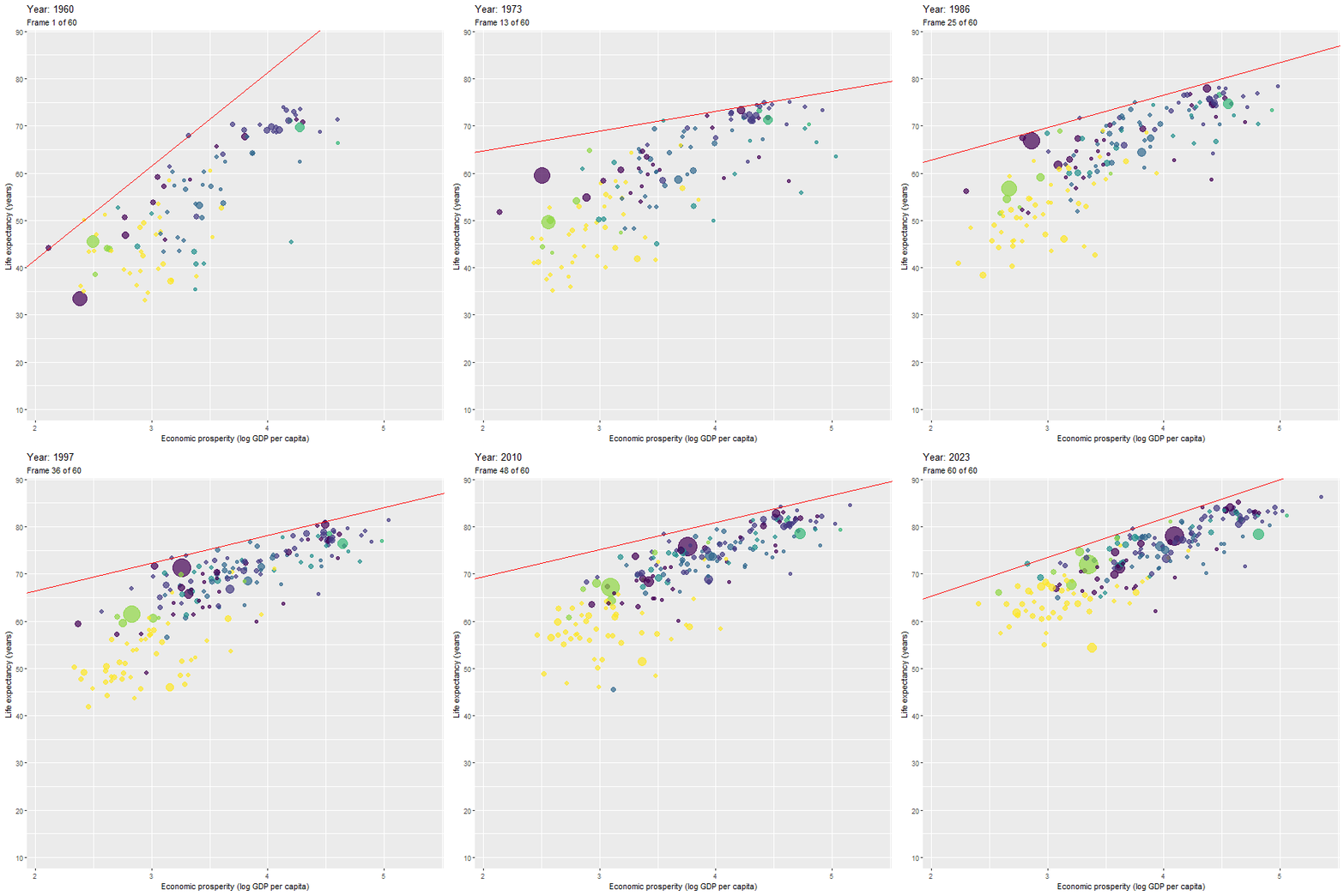
Animation with countries per year with the ceiling line in red.

The animated figure above shows the time trends. In the figure, each data point is a country. The size of a data point refers to the country’s population size, and the color to the geographic region to which it belongs, e.g., yellow for the Sub-Saharan region, and violet for East Asian and Pacific region.

The interpretation of time trends focuses on the change of necessity effect size, ceiling line intercept and ceiling line slope over time. Table 8.1 and Figure 8.2-top-left show the clear trend that necessity effect size reduces over time. This indicates that, over the years, Economic prosperity has become less of a bottleneck for high Life expectancy. Figures 8.2-top-right and 8.2-bottom show that this decrease of effect size is due to the increase of the intercept (upward moving ceiling line) and decrease of the slope (ceiling line flattens).

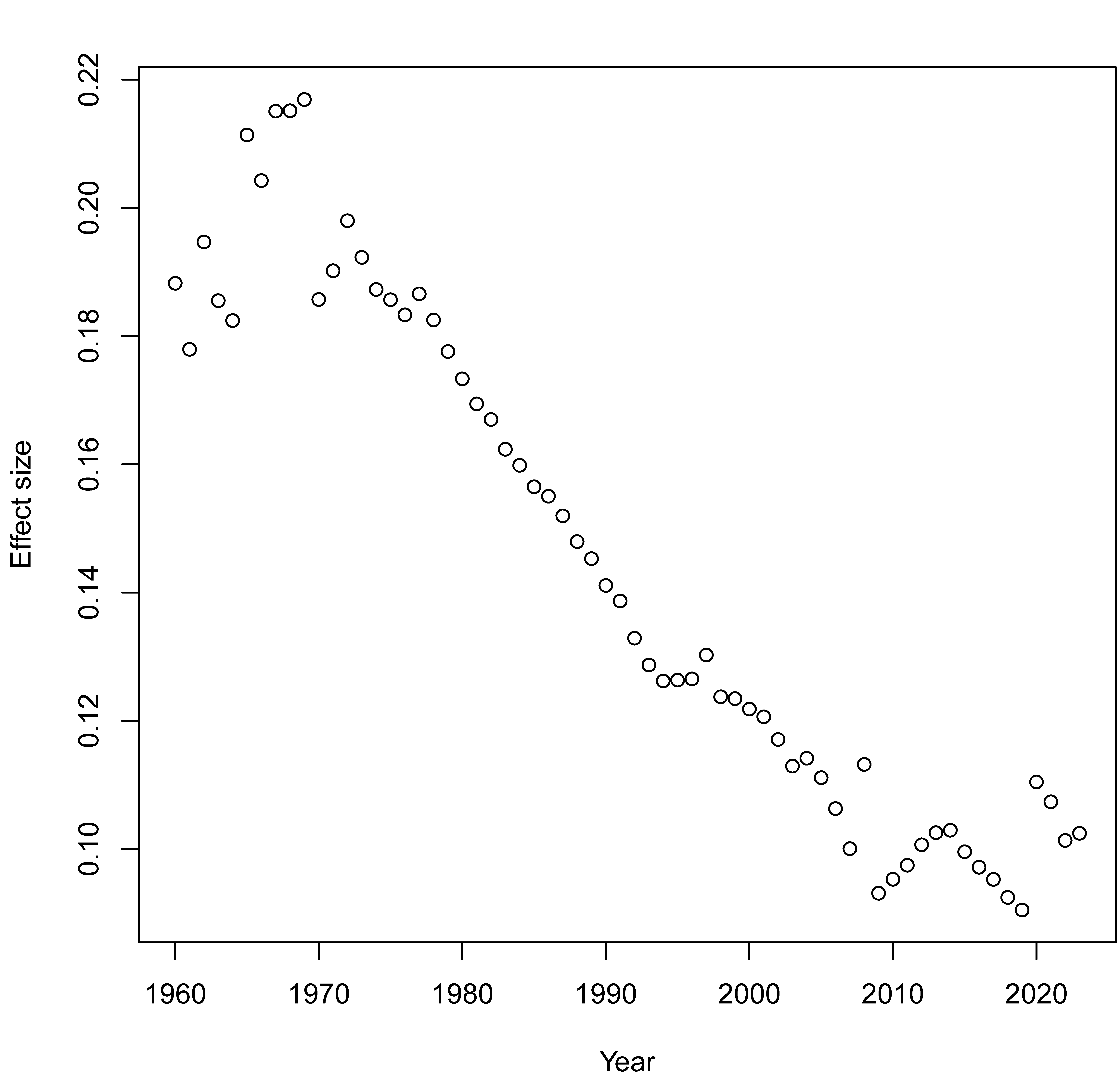
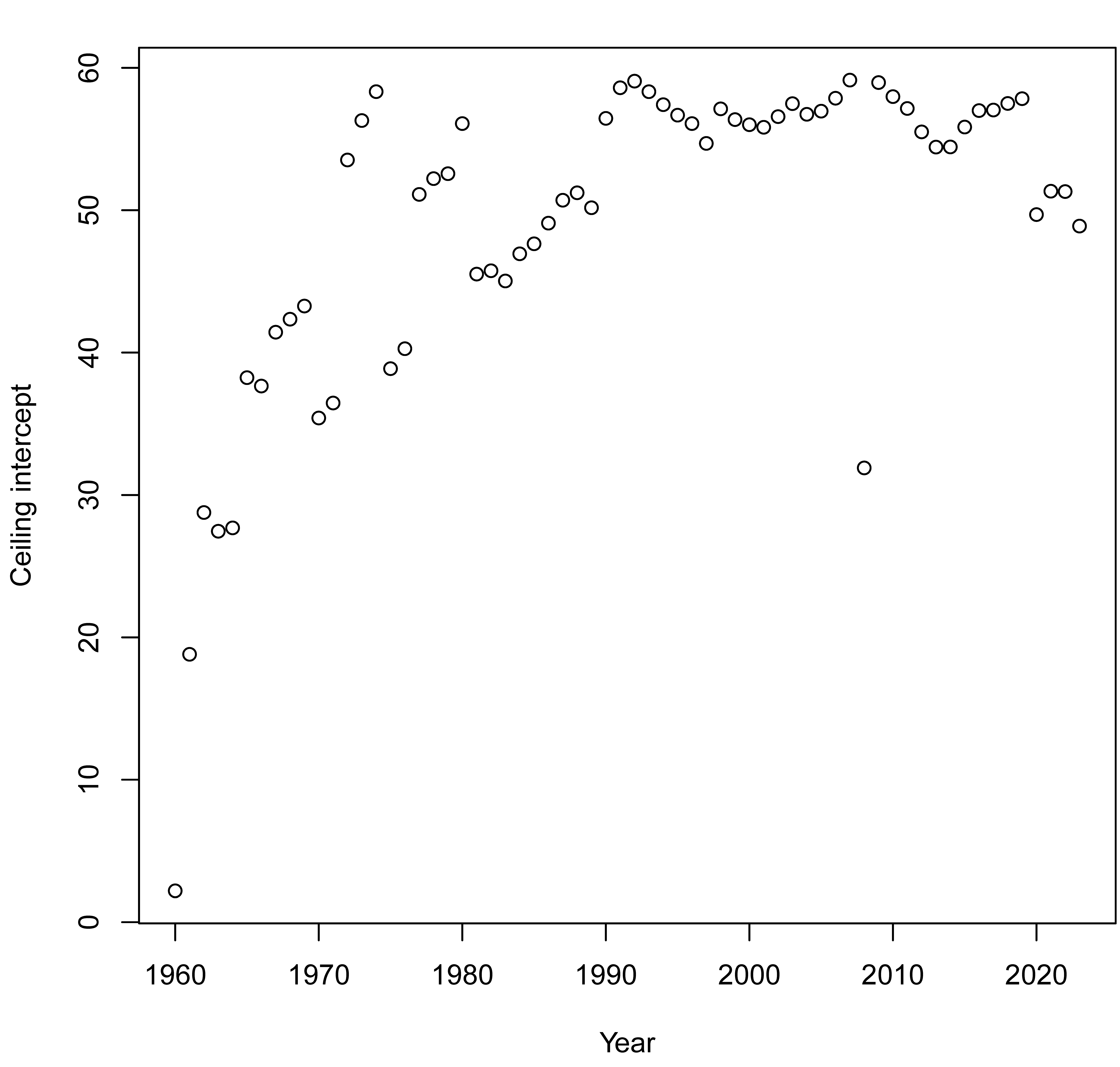
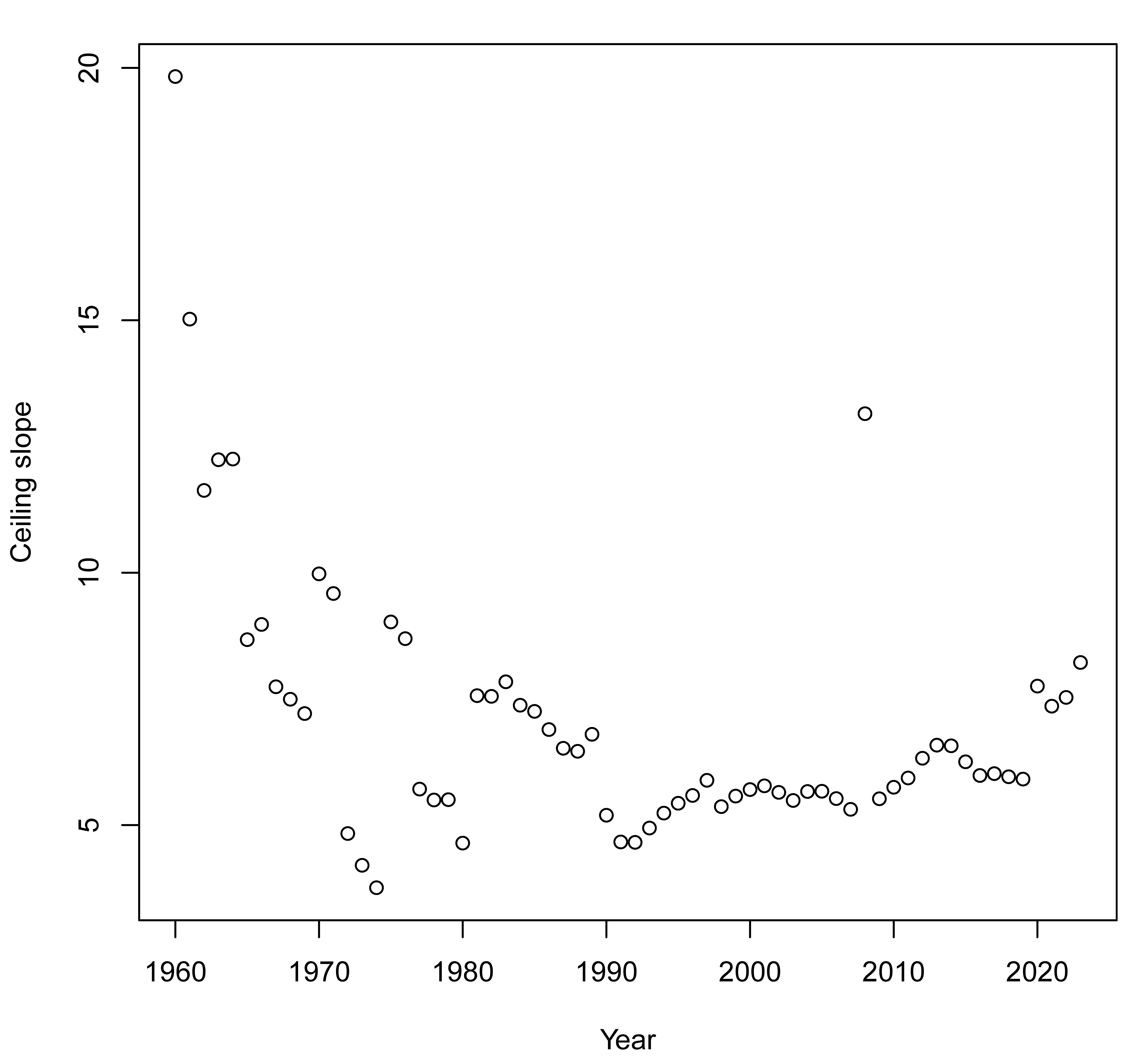
Figure 8.2: Time trends of NCA parameters for the necessity of Economic prosperity for Life expectancy. Top-Left: necessity effect size. Top-Right: ceiling intercept. Bottom: ceiling slope.

Figure 8.3 compares the \(XY\)-plots for the first (1960) and last (2023) year in the dataset and shows that the effect size in 1960 was higher than in 2023.

Figure 8.3: \(XY\)-plot of Economic prosperity and Life expectancy for 1960 (Left) and 2023 (Right).

NCA’s statistical difference test for paired observations (Section 5.3.6) shows that the 0.09 difference between the effect sizes of 1960 and 2023 (0.19 and 0.10, respectively) is statistically significant (\(p\) < 0.001).

In 1960 the maximum life expectancy for an Economic prosperity of 3 (\(10^3\) = 1000 equivalent US dollars) was about 60 years, and in 2023 it was about 75 years. In 2023 compared to 1960, the countries are more clustered near the ceiling, indicating that the difference in Life expectancy between countries diminished, but that a hard border of maximum possible Life expectancy for a given Economic prosperity level remains.

Socio-economic policy practitioners could make new interpretations from these necessity time-trends. For example, in the past, economic prosperity was a major bottleneck for high life expectancy. Currently, most countries are economically prosperous enough for having the possibility of a decent life expectancy of 75 years; if these countries do not reach that level of life expectancy, other factors than economic prosperity are the reason for it. If the trend continues, in the future Economic prosperity may not be a limiting factor for high Life expectancy, because the empty space in the upper-left corner disappears.

8.2.2.3 Time-lagged study

The observed empty space in the upper-left corner could also be the results of reverse causality. In reverse causality \(Y\) existed before \(X\). An empty space in the upper-left corner could then also indicate that a low level of \(Y\) is necessary for a low level of \(X\). This would mean that a low level of Life expectancy is necessary (\(Y\)) for a low level of Economic prosperity \(X\). When forward necessity makes sense, the argument for reverse causality is often weaker but cannot be excluded. With a time-lagged study, reverse causality is less likely when an empty space in the upper-left corner is observed while the \(X\)-score is obtained at time point (\(T_1\)) before the time point (\(T_2\)) of the \(Y\)-score. The lag should be long enough for \(Y\) to develop in the presence of \(X\) and other causal factors. For example, by using a 5-year time-lag the analysis with Economic prosperity in 2018 and Life expectancy in 2023 has a similar empty space in the upper-left corner (Figure 8.4).

Figure 8.4: \(XY\)-plot of Economic prosperity in 2018 and Life expectancy in 2023.

The differences between Figures 8.4 and 8.3-right are minor.

8.2.3 Case study

The case study investigates the phenomena in a small number of cases in their natural environment. Such a design is associated with a small-n qualitative study that allows a rich description of the phenomena. In such a study, relationships are often described in words rather than numerically.

NCA can be applied to a case study design in two ways. First, NCA’s methodology provides the causal logic to describe phenomena. Case studies are often used to explore complex causal relationships within specific contexts, and NCA complements this by introducing the idea that some factors may be necessary (but not sufficient) for an outcome to occur. In this way, NCA helps case investigators to move beyond traditional probabilistic sufficiency cause-effect explanations toward identifying the minimal requirements that must be present for a phenomenon to manifest.

Second, NCA’s data analytic method provides the tools to analyze qualitative data within or across cases. In multiple-case designs, coded evidence from interviews, documents, or observations can be transformed into ordinal or categorical indicators of conditions and outcomes. These can then be used as input scores for NCA to identify which conditions consistently act as enablers or bottlenecks across cases. The results can be interpreted to explain how and why these conditions function as necessary conditions.

If a necessity hypothesis already exists, the case study design can be used to test this hypothesis with the small number of cases. Case studies explicitly designed for testing necessity hypotheses are rare, but implicitly many studies do test such a hypothesis given the way the cases are selected (e.g., Fujita & Kusano, 2020; Harding et al., 2002, see Section 8.3.2 for more details). However, testing a necessity hypothesis as part of an existing case study design, commonly aimed at exploration and theory building, offers a new opportunity for many qualitative studies (e.g., Novales et al., 2025).

When testing a necessity hypothesis with a small number of cases selected from the theoretical domain (deductive case study), a rich description of the context is not required, although it is not objectionable either. The only requirement is that the qualitative data can be scored into levels of the condition and the outcome (e.g., in terms of low, medium, high). Because necessity is independent of other variables, scoring the concepts \(X\) and \(Y\) is enough for testing the hypothesis. Given the small number of cases and their non-random selection, an estimation of \(p\)-values is not feasible. However, the reduced data requirements often allow the analyst to dive deeper into the cases for better understanding the necessity mechanisms, or selecting more than a few cases, bringing the design closer to an observational study (Section 8.2.1). Case selection for testing necessity hypotheses is discussed in Section 8.3.

8.2.4 Experimental study

In an experimental study design, \(X\) is first manipulated and afterwards the effect on \(Y\) is observed, such that the required causal direction is ensured: first \(X\) then \(Y\). This excludes the possibility of reverse causality that \(Y\) occurs before \(X\) (Section 5.7). Whereas uncertainty about the causal direction could be handled with a time-lagged longitudinal study, where the condition is measured at \(T_1\) and the outcome at \(T_2\), such a study can only detect necessity if the outcome has developed during this time period. To have more control, the necessity experiment is an alternative approach for establishing the causal direction when the analyst is uncertain about reverse causality. With this goal in mind, the experiment is useful for testing a necessity hypothesis in the situation that reverse necessity is theoretically plausible.

The experimental setup for a necessity experiment differs from the traditional probabilistic sufficiency experiment in several ways. Whereas in a common experiment \(X\) is manipulated (increased) to produce the presence of \(Y\) on average, in a necessity experiment \(X\) is manipulated (decreased) to produce absence of \(Y\) (assuming a high-high hypothesis or more precisely: assuming that for a desired level of \(y = y_c\), \(x\) must be equal to or larger than \(x_c\)).

The necessity experiment starts with cases with high level of the outcome (\(y ≥ y_c\)) and with high level of condition (\(x ≥ x_c\)), then the condition is removed or reduced (\(x < x_c\)), and it is observed if the outcome has disappeared or reduced (\(y < y_c\)). This contrasts the traditional “average treatment effect” experiment in which the research starts with cases with low outcome (\(y < y_c\)) and with low condition (\(x < x_c\)), then the condition is added or increased (\(x ≥ x_c\)), and it is observed if the outcome has appeared or increased (\(y ≥ y_c\)).

The necessity experiment is conducted as follows:

1. Obtain a representative sample from the population.

2. Check the expected empty corner.

3. Select the entire sample or part of it.

4. Divide this sample randomly into two groups (treatment and control group).

5. Remove (\(x \rightarrow 0\)) or reduce (\(x \rightarrow low\)) the condition in the treatment group.

6. Observe: (1) whether the effect size does not disappear; and (2) whether the outcome reduction in the treatment group is larger than the outcome reduction in the control group. If both are true, necessity is supported.

This necessity experiment ensures the causal direction (first \(X\), then \(Y\)). The randomization between groups ensures that the group constitutions are similar, and that possible time effects (e.g., effect of other disappearing necessary conditions) are controlled for. The possible disappearance/reduction of the outcome due to other necessary conditions happens in both groups; the treatment group must have more outcome disappearance/reduction than the control group.

Below several types of necessity experiments depending on whether \(X\) and \(Y\) are dichotomous or continuous are discussed.

8.2.4.1 Necessity experiment: dichotomous \(X\) and dichotomous \(Y\)

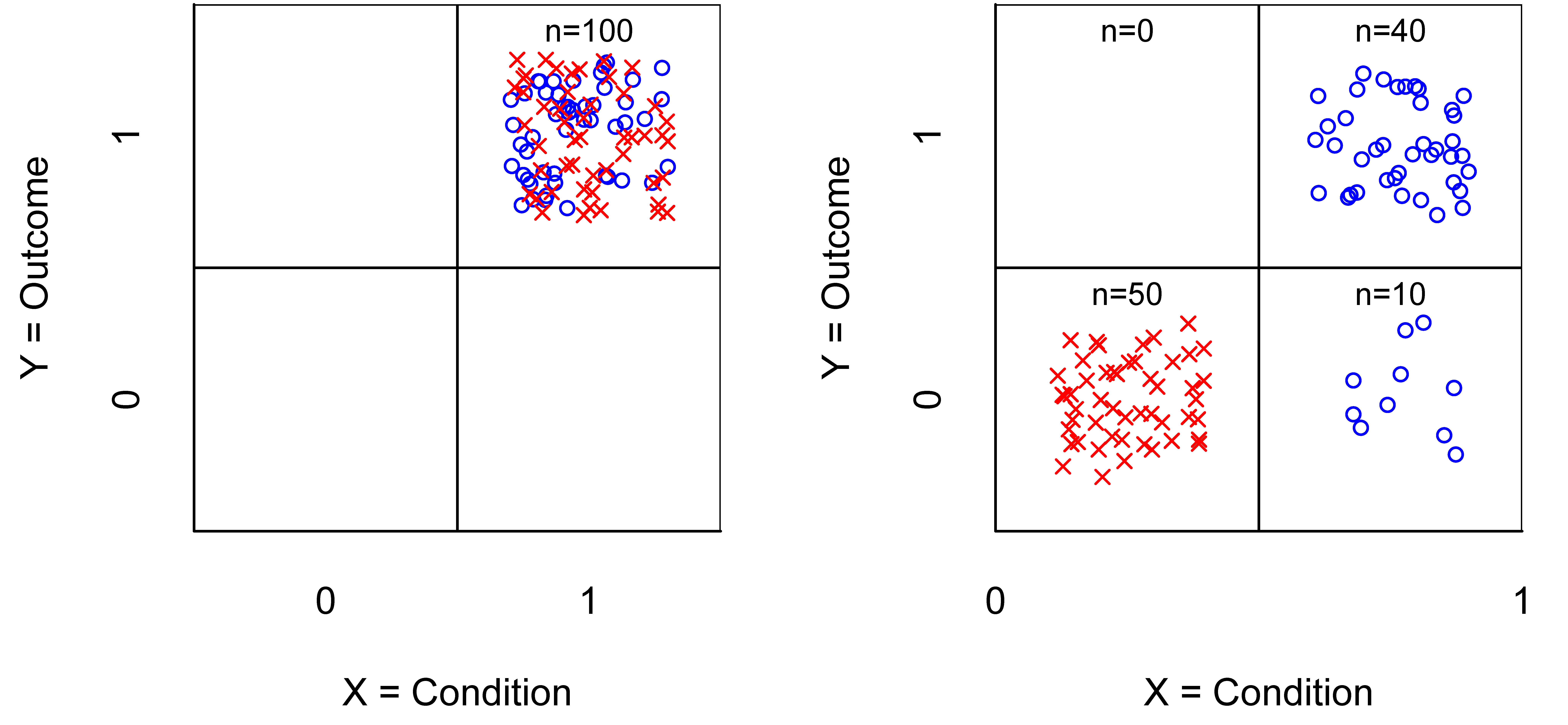
Figure 8.5: \(XY\)-table of the necessity experiment before (Left) and after (Right) manipulation. \(X\) = Condition (0 = no; 1 = yes). \(Y\) = Outcome (0 = no; 1 = yes). = control group. × = treatment group.

For dichotomous variables the experiment to evaluate a high-high necessity hypothesis the steps are conducted as follows:⁷⁶

1. Obtain a representative sample from the population.

2. Observe that expected corner is empty (corner 1).

3. Select the cases of corner 2. The experiment is done with these cases. In Figure 8.5-left it is assumed that 100 cases are available for the experiment.

4. Randomly assign these cases into two groups:

   • Treatment group (symbol ×).
   • Control group (symbol ).

5. Apply the treatment:

   • Treatment group: Remove the condition: \(x\rightarrow\) 0.
   • Control group: Keep the condition: \(x = 1\).

6. Observe the outcome \(Y\) in both groups (Figure 8.5-right):

   • Treatment group: number of cases that move to corner 1.
   • Treatment group: number of cases that move to corner 3.
   • Control group: number of cases that move to corner 4.
   • Control group: number of cases that remain in corner 2.

If all treatment cases have moved from corner 2 to corner 3, but not to corner 1, and if not all control cases have moved from corner 2 to corner 4 (because another necessary condition disappeared during the manipulation) there is evidence that \(X\) is necessary for \(Y\). If treatment cases have moved from corner 2 to corner 1, this indicates that \(Y\) can occur without \(X\) and that \(X\) is not necessary for \(Y\). If control cases have moved from corner 2 to corner 4, this suggests that there is a time effect. This is not a problem for concluding that \(X\) is necessary for \(Y\) as long as not all control cases have moved to corner 4.⁷⁷

8.2.4.2 Necessity experiment: dichotomous \(X\) and continuous \(Y\)

Figure 8.6 illustrates the situation when the condition is dichotomous and the outcome is continuous. Before the manipulation the condition is present (\(x\) = 1). The \(y\)-values include the maximum value of the outcome (\(y\) = 1). Necessity is supported when after the manipulation (\(x \rightarrow 0\)) the maximum value in the treatment group is reduced to a value of \(y = y_c\), resulting in an empty upper-left corner of the \(XY\)-plot. The necessary condition can be formulated as \(x = 1\) is necessary for \(y \geq y_c\). The necessity effect size is the empty area divided by the scope. In this example the effect size = 0.18.

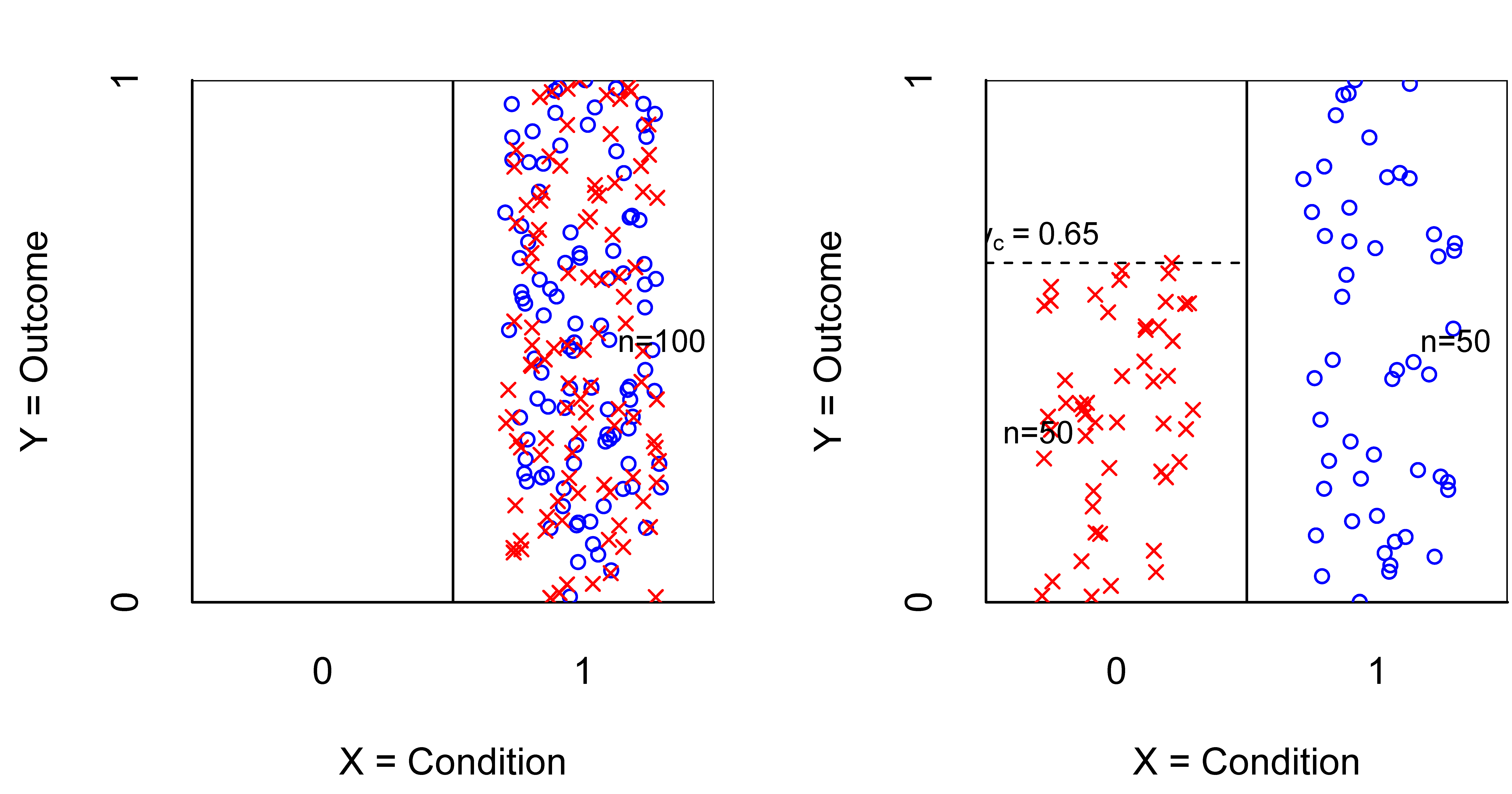
Figure 8.6: \(XY\)-plot of the necessity experiment with a continuous outcome and a dichotomous condition before (Left) and after (Right) manipulation. \(X\) = Condition (0 = no, 1 = yes). Y = Outcome between 0 and 1. = control group. × = treatment group. \(y_c\) is the ceiling value of \(Y\) for \(x\) = 0.

8.2.4.3 Necessity experiment: continuous \(X\) and dichotomous \(Y\)

Figure 8.7 illustrates the situation when the condition is continuous and the outcome is dichotomous. Before the manipulation, the condition is present: \(x \geq x_{high}\), where \(x_{high}\) is a value above the presumed necessity level \(x = x_c\). The treatment reduces the value of \(x\) of all treatment cases. Some cases may end below \(x = x_{high}\) but above \(x = x_{c}\). Since the bottleneck value \(x_c\) is not reached, these cases have \(y\) = 1. Other treatment cases have new \(x\)-values below the necessity value \(x\) = \(x_c\). The latter group of cases will then end up in the lower-left corner with \(y = 0\). Necessity is supported when after manipulation no cases with \(y = 1\) exist with \(x < x_c\). In other words, all cases with \(x < x_c\) should be located in the lower-left corner. The necessary condition can be formulated as \(x \geq x_c\) is necessary for \(y = 1\).

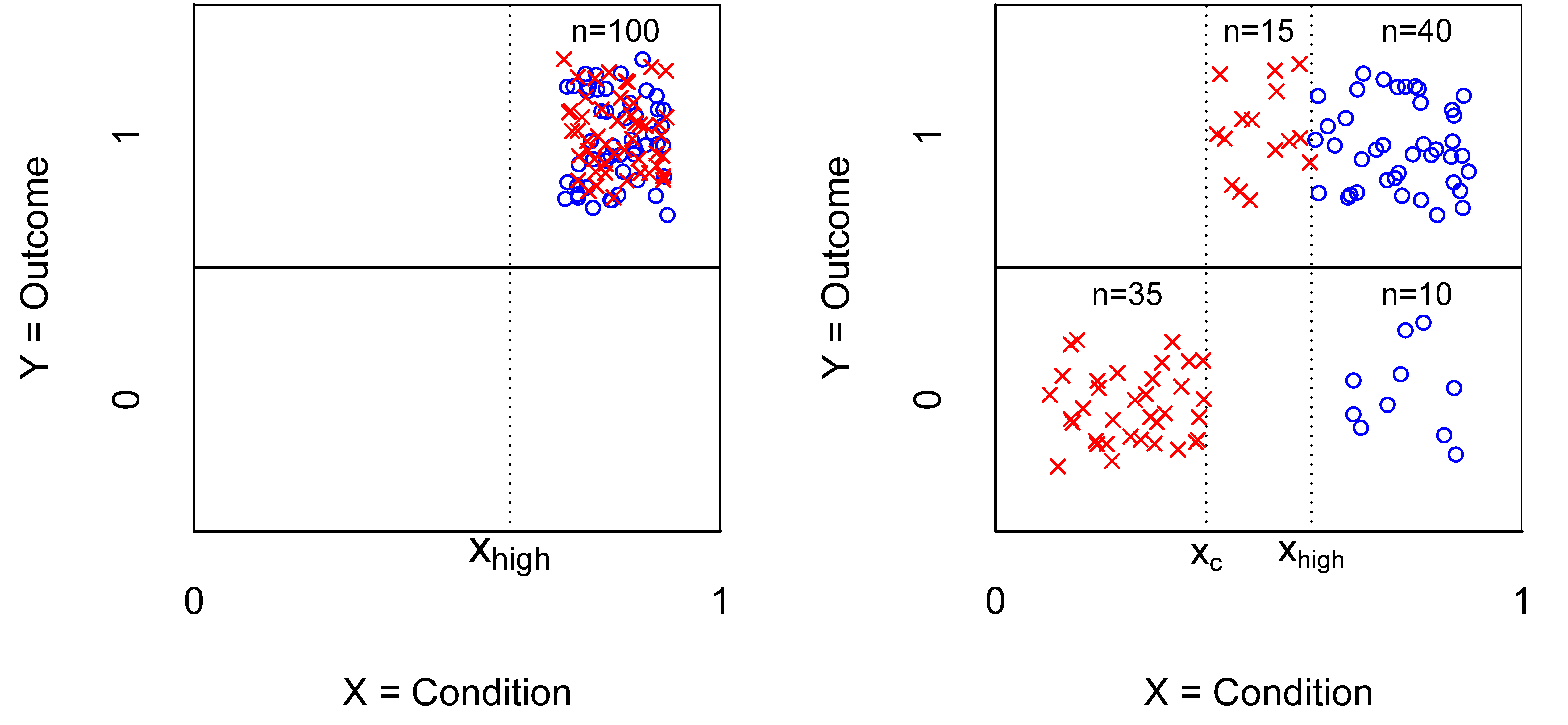
Figure 8.7: \(XY\)-plot of the necessity experiment with a continuous condition and a dichotomous outcome before (Left) and after (Right) manipulation. \(X\) = Condition (0 = no, 1 = yes). \(Y\) = Outcome between 0 and 1. = control group. × = treatment group. \(x_c\) is ceiling value of \(x\)-value for \(y\) = 1. \(x_{high}\) is the minimum \(x\)-value for selecting cases with \(y\) = 1.

8.2.4.4 Necessity experiment: continuous \(X\) and continuous \(Y\)

In a necessity experiment with a continuous condition and a continuous outcome, the starting point is the existence of an empty area in the upper-left corner of the \(XY\)-plot (Figure 8.8-left). The manipulation consists of reducing the level of the condition in the treatment group but not in the control group. Necessity is supported when after the manipulation no cases enter the empty zone. This is shown in Figure 8.8-right, where the necessity effect size before manipulation (0.25) stays intact after manipulation.

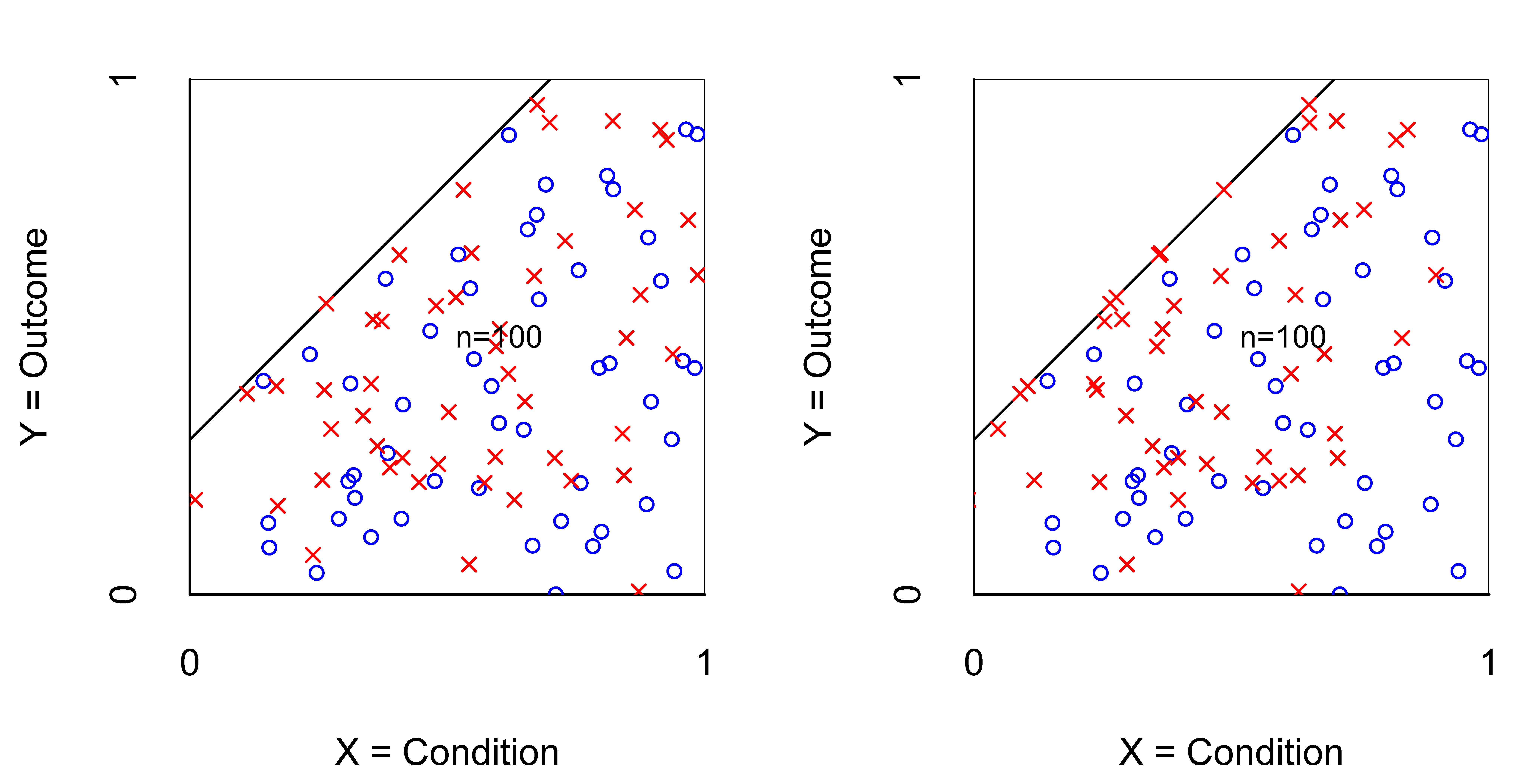
Figure 8.8: \(XY\)-plot of a necessity experiment with a continuous condition and outcome before (Left) and after (Right) manipulation (reducing \(X\)). Effect size remains after manipulation. = control group. × = treatment group.

However, when cases enter the empty zone, the necessity is reduced (smaller effect size) or rejected (no empty space). Figure 8.9-right shows an example of a reduction of the necessity effect size from 0.25 to 0.15.

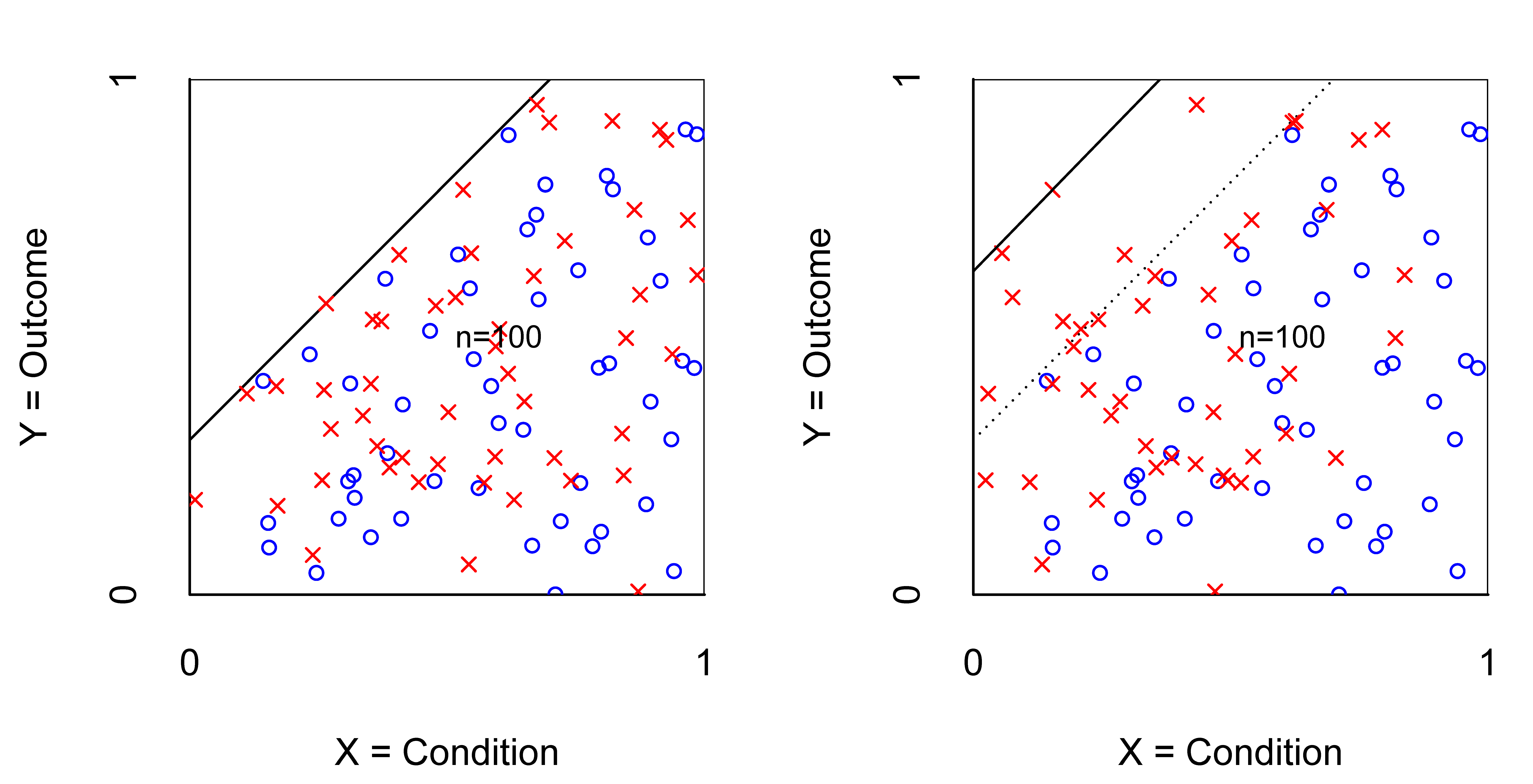
Figure 8.9: \(XY\)-plot of a necessity experiment with continuous conditions and outcome before (Left) and after (Right) manipulation (reducing \(X\)). Effect size reduces after manipulation. = control group. × = treatment group.

Figure 8.10 displays an example of an experiment in which a necessity effect disappears after experimental manipulation. In such cases, the necessity hypothesis should be rejected.

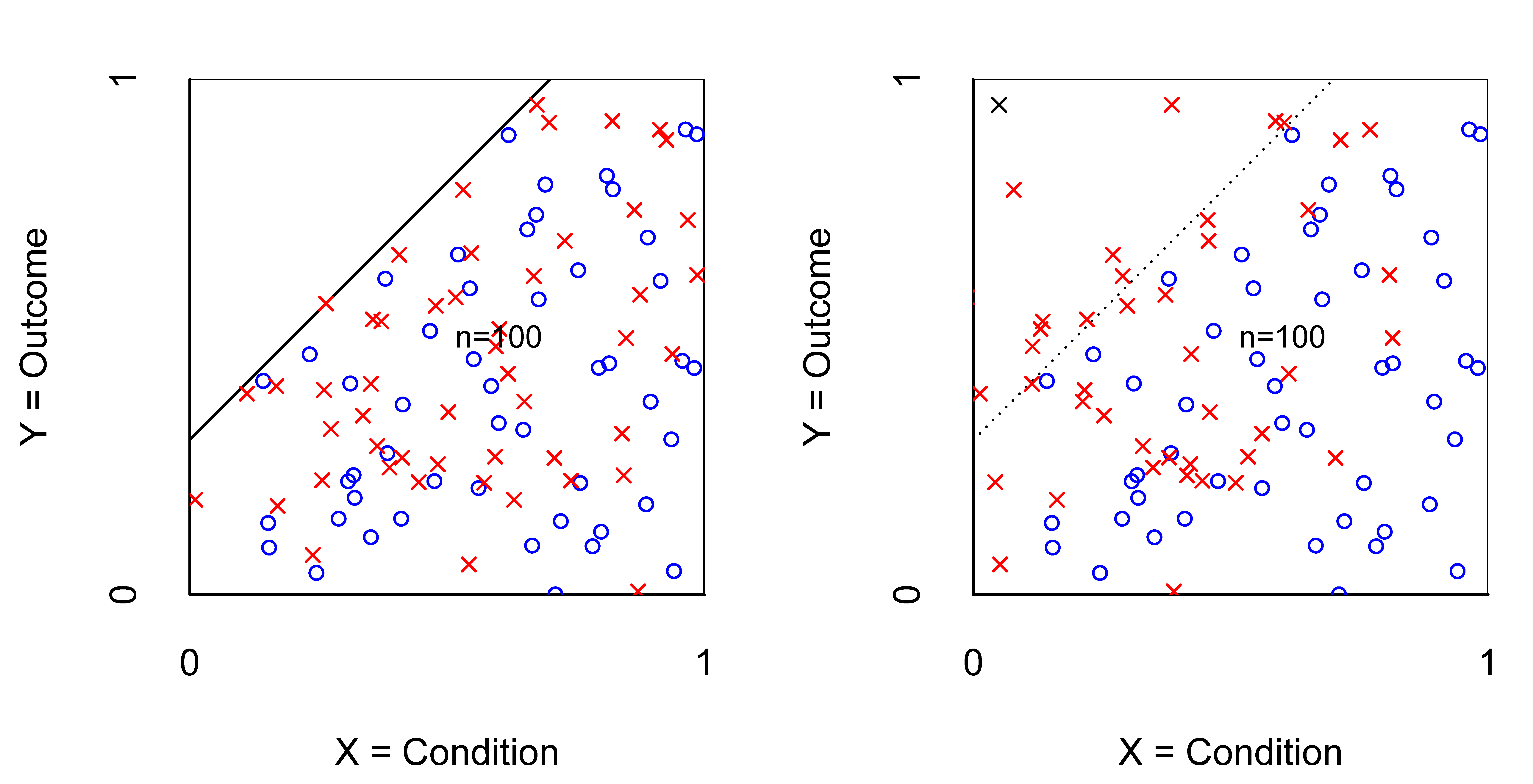
Figure 8.10: \(XY\)-plot of an experiment to challenge necessity with continuous condition and outcome before (Left) and after (Right) manipulation of reducing \(X\). Effect size disappears after manipulation. = control group. × = treatment group.

In situations with a poorly covered sample, before manipulation the necessary condition may not be visible as an empty space in the upper-left corner because only cases are selected where the conditions are satisfied. After manipulation, the new scope (empirical or theoretical) is extended and a hidden empty space becomes visible. (Figure 8.11).

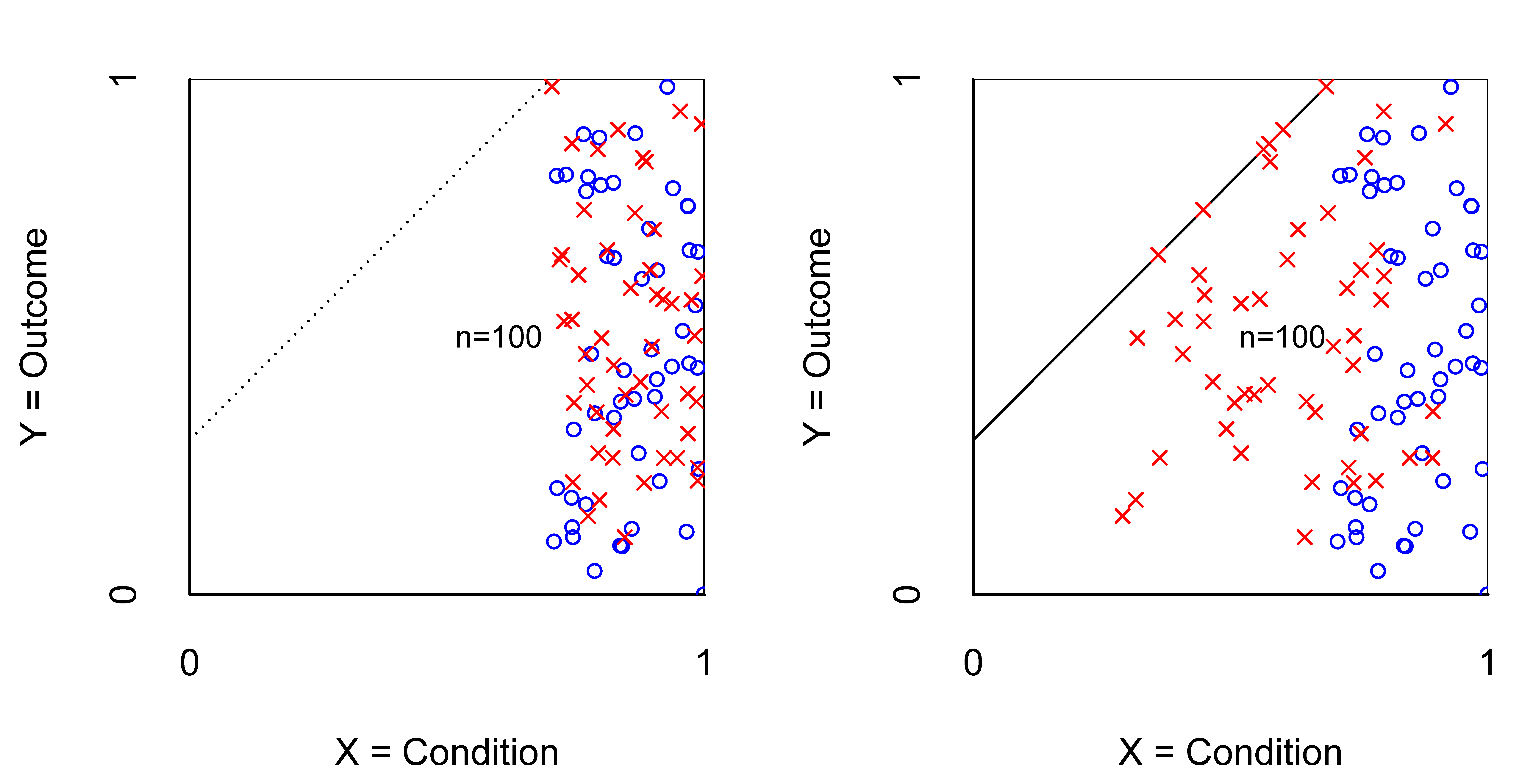
Figure 8.11: \(XY\)-plot of a necessity experiment with a continuous condition and outcome before (Left) and after (Right) manipulation (reducing \(X\)). Effect size appears after manipulation. = control group. × = treatment group.

8.3 Sampling and selection of cases

After the choice of the type of study design, cases must be obtained from the theoretical domain where the necessity hypothesis is supposed to hold. The cases are used to test the hypothesis. In general it is a good strategy to select as many cases as possible. However, necessity theory may be broadly applicable in the theoretical domain consisting of many cases. If not all cases can be selected, a thoughtful selection must be done. NCA offers two types of case selection: large-n sampling for a quantitative study and small-n case selection for a qualitative study.

8.3.1 Large-n sampling

The goal of large-n sampling for a quantitative NCA study is to have a sample that is representative of a defined population from the theoretical domain. Usually, different populations where the cases have some relevant common characteristic (e.g., from the same country) could be selected. Since the theoretical domain may not be homogeneous, different populations could have different effect sizes, although the hypothesis claims that overall necessity exists for all cases. The selection of the population itself is not guided by statistical principles and can often be done for convenience. However, after the population is selected from the theoretical domain, random sampling of a large sample helps to ensure that the population is well-covered in the sample and that findings based on the sample can be statistically generalized to the population (inferential statistics). A possible approach to achieve this is to have a sampling frame (list of cases) of the population and to select cases randomly from this list. This ideal sampling approach contrasts with the more common approach of convenience sampling where cases are selected from the population for the analyst’s convenience, for example because the analyst has easy access to the cases. With such a sampling procedure, the sample may not be representative of the population, which can lead to biased effect size estimates and invalid \(p\)-values. The decision on the size of the sample depends on available resources and other practical factors. The minimum required sample size can be guided by the expected power of the study. Power refers to the minimum required sample size such that an existing relevant necessity effect size can be detected with high probability (Section 5.6).

8.3.2 Small-n case selection

It is possible to test a necessity hypothesis with a small number of cases, even with one case (e.g., Dul & Hak, 2008). In qualitative studies, usually a small number of cases is selected with a certain purpose in mind.⁷⁸ For testing a necessity hypothesis, the purpose of sampling is to have cases where the outcome is present (\(Y = 1\)) or the condition is absent (\(X = 0\)). After selecting such cases, it is observed if the condition is present (\(X = 1\)) or the outcome is absent (\(Y = 0\)), respectively. If the condition is absent in cases where the outcome is present, or the outcome is present in cases where the condition is absent, the necessary condition hypothesis is rejected for these cases. This type of purposive sampling in small-n studies is possible with a deterministic view on necessity (no exceptions) and when the conditions and the outcome have dichotomous scores (e.g., absent/present, low/high). Since according to the hypothesis necessity applies to each single case in the theoretical domain, a single case can be selected for the test. If necessity is rejected in that single case, the deterministic version of the necessity hypothesis is rejected. However, support for necessity based on only one or a few cases is often not convincing for a conclusion about the entire theoretical domain. Other cases that falsify the necessary condition hypothesis may not have been selected. Following replication logic, the confidence in a hypothesis increases when more cases do not falsify the hypothesis.

Purposive selection of cases for testing a necessity hypothesis was used implicitly in a study by Fujita & Kusano (2020) of highly controversial visits by Japanese Prime Ministers (PM’s) to the Yasukuni Shrine. Three necessary conditions were expected: a conservative ruling party, a government enjoying high popularity, and Japan’s perception of a Chinese threat. They tested these hypotheses by selecting all five cases where the outcome was present (\(Y = 1\), PM’s who visited the shrine) from all 22 cabinets between 1986 and 2014. They found that the three conditions were present in all cases (\(X = 1\)) suggesting support for necessity, at least no rejection. Additionally, they selected the 17 cases where at least one potential necessary condition was absent (\(X = 0\)) and found that in these cases no visit occurred (\(Y = 0\)), giving further support for necessity.

In another small-n qualitative study, Harding et al. (2002) studied rampage school shootings in the USA. They first identified five potential necessary conditions: gun availability, cultural script (a model why the shooting solves a problem), perceived marginal social position, personal trauma, and failure of a social support system.⁷⁹ Subsequently, they tested the necessary conditions with two cases of school shooting (\(Y = 1\)) and found support for necessity (non-rejection) because the five conditions were present in these cases (\(X = 1\)).

Note that this approach of selecting a small number of cases for testing a necessity hypothesis is used in Chapter 7 as part of thought experiments to evaluate a preliminary necessity hypothesis based on existing knowledge (Section 7.5.2).

8.3.3 Replication

Since the necessity hypothesis is assumed to hold for all cases in the entire theoretical domain and the samples or selected cases that are used for testing the hypothesis are only a subset of the theoretical domain, replication studies with other cases are needed. Replication is re-testing the hypothesis with new data (Köhler & Cortina, 2023). A single shot study is not conclusive about a hypothesis in the entire theoretical domain. A next study should select cases from other parts of the theoretical domain, i.e., other samples from the sample population and samples from other populations for large-n sampling, or other cases for small-n case selection. Although a hypothesis can never be proven correct, the confidence in its correctness increases if repeated tests with different samples/cases fail to falsify the hypothesis.

8.4 Measurement

After the cases are sampled/selected, the \(X\) and \(Y\) characteristics of each case must be measured. In NCA the scores are often numeric (numbers, quantitative data) but words or letters (qualitative data) can also be used to represent levels of concepts (e.g., high or low). The goal of measurement is to obtain valid and reliable scores of the concepts \(X\) (the conditions) and \(Y\) (the outcome) that are defined in the necessity hypothesis. Scores are valid when they represent the value of a concept (measuring what you want to measure) and reliable when they are consistent under identical circumstances.

8.4.1 Quantitative data

Quantitative data are data expressed by numbers where the numbers are scores (values or levels) with a meaningful order and meaningful distance. Scores can have two levels (dichotomous, e.g., 0 and 1 ), a finite number of levels (discrete, e.g., 1,2,3,4,5) or an infinite number of levels (continuous, e.g., 1.8, 9.546, 306.22).

NCA can be used with any type of quantitative data. It is possible that a single indicator represents an \(X\) or \(Y\) concept. Then this indicator score is used to score the concept. For example, in a questionnaire study where a subject or informant is asked to score conditions and outcomes with seven-point Likert scales, the scores are one of seven possible (discrete) scores.

It is also possible that a construct that is built from several indicators is used to represent the concept of interest. Separate indicator scores are then summed, averaged or otherwise combined (aggregated), for example for scoring a formative index. It is also possible to combine several indicator scores statistically, for example by using the factor scores resulting from factor analysis, or construct scores of latent variables resulting from a measurement model.

8.4.2 Qualitative data

Qualitative data are data expressed by names, letters or numbers without a quantitative meaning. For example, gender can be expressed with names (male, female, other), letters (m, f, o) or numbers (1, 2, 3). Qualitative data are discrete and usually have no order between the scores (e.g., names of people) or if there is an order, the distances between the scores are unspecified (e.g., low, medium, high). Although with qualitative data a quantitative NCA (with the NCA software for R) is not possible, it is still possible to apply NCA in a qualitative way using visual inspection of the \(XY\)-table or plot.

When \(X\) and \(Y\) of cases are scored qualitatively, for example \(X\) = A,B, or C, and \(Y\) = no or yes, the corresponding \(XY\)-table has 6 cells where a case has a position in one of the cells. The hypothesis may be that B is necessary for yes. The analyst can inspect which \(X\)-score can reach that \(Y\)-score. When the logical order of the condition is absent, the position of the empty space can be in any upper cell (left corner, middle or right; assuming the hypotheses that high \(X\) is necessary for high \(Y\)). When a logical order exists between the qualitative \(X\)-scores, the empty space is in the upper-left corner. In both cases the size of the empty space is arbitrary and no meaningful effect size can be calculated. However, when \(Y\) is quantitative, the distance between the highest observed \(Y\)-score and the next-highest observed \(Y\) score could be an indication of the constraint of \(X\) on \(Y\).

8.4.3 Set membership data

NCA can be used with set membership scores. This is often done when NCA is combined with QCA (Section 11.5). In QCA ‘raw’ variable scores are ‘calibrated’ into set membership scores with values between 0 and 1. A set membership score indicates to what extent a case belongs to the set of cases that have a given characteristic. In crisp set QCA the scores are dichotomous (0 or 1), and in fuzzy set QCA the scores are discrete or continuous between 0 and 1.

8.5 Dataset

After the measurements are done, the \(X\)- and \(Y\)-scores are integrated into a dataset. An appropriate format is having cases as rows and conditions and outcome as columns, where the first row (header) consists of the names of the conditions and outcome, and the first column the names of the cases.

Table 8.2 shows the dataset of the example used in Chapter 9 that is part of the NCA software.

Table 8.2: Example dataset nca.example from the NCA software in R.

	Individualism	Risk taking	Innovation performance
Australia	90	84	50.9
Austria	55	65	52.4
Belgium	75	41	75.1
Canada	80	87	81.4
Czech Rep	58	61	14.5
Denmark	74	112	116.3
Finland	63	76	173.1
France	71	49	77.6
Germany	67	70	109.5
Greece	35	23	12.0
Hungary	80	53	5.4
Ireland	70	100	62.3
Italy	76	60	19.7
Japan	46	43	171.6
Mexico	30	53	1.2
Netherlands	80	82	68.7
New Zealand	79	86	14.9
Norway	69	85	75.1
Poland	60	42	3.5
Portugal	27	31	11.1
Slovak Rep	52	84	3.5
South Korea	18	50	42.3
Spain	51	49	17.3
Sweden	71	106	184.9
Switzerland	68	77	149.7
Turkey	37	50	1.4
UK	89	100	79.4
USA	91	89	214.4

8.5.1 Archival data

NCA needs a dataset with \(X\)- and \(Y\)-values as input to empirically test the hypothesis that \(X\) is necessary for \(Y\). Often, new data on \(X\) and \(Y\) are gathered for conducting such a test. This requires a decision about the study design, the sampling/selection of cases, and the measurement of \(X\) and \(Y\). The quality of NCA depends on the quality of conducting these steps. However, it is also possible that an existing dataset is used. It may be that data on \(X\) and \(Y\) have already been tested for other purposes in previous studies. For example, a large number of datasets have been used with the goal of testing probabilistic sufficiency relationships (e.g., average effect of \(X\) on \(Y\) using regression analysis). If existing datasets contain \(X\)- and \(Y\)-scores of cases that are part of the theoretical domain, and if study design, sampling/case selection and measurement meet the quality criteria, the datasets from earlier studies may be useful for testing the necessity hypothesis. Given the trends toward open science, relevant datasets for testing necessity hypotheses are available, for example the World Bank dataset used in Section 8.2.2.When using archival data, the origins of the data should be evaluated and acknowledged, possible adaptations of \(X\)- and \(Y\)-scores should be justified and reported, and relevant earlier studies that use the same data should be evaluated and referenced to ensure accumulation of knowledge (Dul et al., 2024). In a multimethod study that combines NCA with other methods (Chapter 11), data that were collected for the other method may be re-used for NCA.

8.5.2 Data transformation

In quantitative (statistical) studies, data are often transformed before the actual analysis is done. For example, in machine learning, cluster analysis and multiple regression analysis, data are often standardized. The sample mean is subtracted from the original score and divided by the sample standard deviation to obtain the z-score: \(X_{new} = (X - X_{mean}) / SD\). This allows, for example, a comparison of the regression coefficients of the variables, independently of the variable scale. Min-max normalization is another type of data transformation: \(X_{new} = (X - X_{min}) / (X_{max} - X_{min})\). Such normalized variables have scores between 0 and 1. Transforming original scores into z-scores or min-max normalized scores are both examples of a linear transformation.

In principle, NCA does not need data transformation. The effect size is already normalized between 0 and 1 and allows comparison of effect sizes of different variables. Also, NCA does not make assumptions about the distribution of the data. Furthermore, interpretation of the results with original data is often easier than the interpretation of the results with transformed data as the original data may have a more direct meaning than the transformed data. If, nevertheless, the analyst wishes to transform data, a linear transformation (or in general an affine transformation) does not affect NCA’s estimation of the effect size or the \(p\)-value (Appendix D).

However, a non-linear data transformation as is often done in quantitative (statistical) studies affects NCA’s estimation of effect size and \(p\)-value and is normally not acceptable for NCA. The transformation may change the cases that are used to establish the ceiling line, and this will affect the effect size. This can happen, for example, when data with a skewed distributed are log-transformed to obtain more normally distributed data. This is relevant when a statistical approach assumes normally distributed data, but this is not a requirement in NCA. Calibration in QCA is another example of a non-linear transformation. Original variable scores (‘raw scores’) are transformed into set membership scores, often using a logistic function (‘s-curve’). Calibration is needed in QCA as a set-theoretic method, but not in NCA, that can also handle raw scores.

Non-linear transformations should be avoided in NCA, unless there is a good reason for it. Such a good reason can be that a non-linear transformed original score is the valid representation of the concept of interest (\(X\) or \(Y\) in the necessity hypothesis). For example, the concept of a country’s economic prosperity may be expressed as the log-transformed GDP (Section 8.2.2.1). In QCA, the calibration process can justify the non-linear transformation of the original data. However, the general advice is to refrain from non-linear data transformation when the original data represent the concepts of interest, and only to transform data non-linearly when this is needed to validly capture the concept of interest.

References

Dul, J., & Hak, T. (2008). Case Study Methodology in Business Research. Routledge. https://www.routledge.com/Case-Study-Methodology-in-Business-Research/Dul-Hak/p/book/9780750681964

Dul, J., Raaij, E. van, & Caputo, A. (2024). Advancing scientific inquiry through data reuse: Necessary Condition Analysis with archival data. Strategic Change, 33(1), 35–40. https://doi.org/10.1002/jsc.2562

Fujita, T., & Kusano, H. (2020). Denial or history? Yasukuni visits as signaling. Journal of East Asian Studies, 20(2), 291–316. https://doi.org/10.1017/jea.2020.2

Harding, D. J., Fox, C., & Mehta, J. D. (2002). Studying rare events through qualitative case studies: Lessons from a study of rampage school shootings. Sociological Methods & Research, 31(2), 174–217. https://doi.org/10.1177/0049124102031002003

Jaiswal, M., & Zane, L. J. (2022b). Drivers of sustainable new technology diffusion in national markets: The case of electric vehicles. Thunderbird International Business Review, 64(1), 25–38. https://doi.org/10.1002/tie.22243

Katz, J. (2001). Analytic induction. In N. J. Smelser & P. B. Baltes (Eds.), International Encyclopedia of the Social & Behavioral sciences (Vol. 1, pp. 480–484). Elsevier Oxford, UK. https://doi.org/10.1016/B0-08-043076-7/00774-9

Köhler, T., & Cortina, J. M. (2023). Constructive replication, reproducibility, and generalizability: Getting theory testing for JOMSR right. Journal of Management Scientific Reports, 1(2), 75–93. https://doi.org/10.1177/27550311231176016

Novales, A., Mocker, M., Van Heck, E., & Dul, J. (2025). Realizing desired effects from digitized product affordances: A case study of key inhibiting factors. Decision Support Systems, 189, 114365. https://doi.org/10.1016/j.dss.2024.114365

Robinson, W. S. (1951). The logical structure of analytic induction. American Sociological Review, 16(6), 812–818. https://doi.org/10.2307/2087508

Znaniecki, F. (1934). The Method of Sociology. Farrar & Rinehart.

---

72. The NCA analysis is done with the C-LP ceiling line (Section 4.4), which is a linear ceiling line that has no observations above it. The effect sizes for the pooled data with the two ceiling techniques are 0.10 (p < 0.001) and 0.14 (p < 0.001), respectively.↩︎

73. There is also a well-known positive average relationship (imaginary line through the middle of the data), but this average trend is not considered here. Furthermore, the lower-right corner is empty as well. This suggests that a low level of Economic prosperity is necessary for a low level of Life expectancy. However, this low-low necessity relationship was not claimed in the hypothesis that is tested here. The necessity of low \(X\) for low \(Y\) can be evaluated with the corner = 4 argument in the nca_analysis function of the NCA software (Appendix B)↩︎

74. The time trend expectation can be included in the causal explanation of the hypothesis, see Section 7.5.3.↩︎

75. Only the C-LP ceiling technique is used. For making the NCA results comparable per year, the theoretical scope for each year is the scope of the pooled data (based on the absolute minima and maxima of empirically observed Economic prosperity and Life expectancy in the data).↩︎

76. Convention in this book for corner numbers: 1 = upper-left; 2 = upper-right; 3 = lower-left; 4 = lower-right.↩︎

77. Note that an odds ratio (OR) is often used to estimate the average effect when \(X\) and \(Y\) are dichotomous. The odds ratio summarizes how much more likely (in terms of odds) the outcome is to be absent in the treatment group (where \(X\) is removed) compared to the control group (where \(X\) is retained). The mathematical formula for the odds ratio is \(OR = \frac{c3 / c1}{c4 / c2} = \frac{c3 \cdot c2}{c1 \cdot c4}\) where \(c1\), \(c2\), \(c3\), and \(c4\) refer to the number of cases in corner 1, corner 2, corner 3, and corner 4, respectively. After the treatment, \(c2\) is the number of cases in the control group with outcome success, \(c4\) is the number of cases in the control group with outcome failure (spontaneous decay), \(c1\) is the number of cases in the treatment group with outcome success (success remains after removing \(X\)), and \(c3\) is the number of cases in the treatment group with outcome failure. With an observed data pattern of an empty space in corner 1, the odds ratio is infinite, regardless of the distribution of the cases in the control group: \((50/0)/(10/40) = \infty\). This situation is called “perfect separation” and is considered a problem for average effect statistical analysis. A common advice is to remove the \(X\) from further analysis. However, \(X\) is a very important predictor of the outcome: the perfect predictor ensures absence of the outcome when \(X\) is absent: a necessary condition.↩︎

78. For example typical cases that represent a wider population of cases, deviant cases that are unusual, or maximum variation cases to ensure maximum variation of a certain characteristic.↩︎

79. They identified these five potential necessary conditions not by using existing knowledge (Section 7.2) but by first conducting an inductive case study. The authors selected two cases where the outcome was present (school shooting) and observed common factors. The two cases were different from the cases used for testing the hypothesis. Identifying “important” factors in this way has a long tradition in explorative and theory-building case study designs. For example, Znaniecki (1934) introduced ‘analytic induction’ for finding causal relationships. This method identifies common characteristics in cases where the outcome is present, thus identifies potential necessary conditions (Katz, 2001; W. S. Robinson, 1951).↩︎