11 Multimethod studies

11.1 Summary of this chapter

The previous chapters focus on NCA as a standalone methodology and method. This chapter explores how NCA can be applied in combination with other methods. First, a distinction is made between method-triangulation studies that use multiple methods with the same causal perspective, and causal-pluralism studies using multiple methods with distinct causal perspectives (Section 11.2). Next, causal-pluralism multimethod studies that combine NCA with regression-based methods are discussed, showing that NCA can provide insights beyond average effects. With the NCA-Extended Regression Table (NERT) tool, the results can be compared (Section 11.3). This is followed by discussing how NCA can be combined with a specific regression-based method, structural equation modeling (SEM). To compare the results, the Bottleneck Importance Performance Map Analysis (BIPMA) tool is provided (Section 11.4). Both tools acknowledge the different causal perspectives, while facilitating the combined interpretation of results. Subsequently, multimethod studies that combine NCA with Qualitative Comparative Analysis (QCA) are discussed (Section 11.5). Section 11.6 shows how NCA insights on necessity-in-degree can provide additional insights for QCA’s necessity and sufficiency analyses. For the combined interpretation of NCA’s necessity results and QCA’s sufficiency results, the NCA-Extended Solution Table (NEST) tool is provided.

11.2 Method-triangulation versus causal-pluralism

Studies that apply multiple methods are commonly praised for their ability to produce deeper or more robust insights than studies that rely on a single method. For example, a qualitative analysis of interview data can enrich a quantitative analysis of questionnaire data, and vice versa, or regression approaches with different model specifications or parameter estimation techniques may make conclusions more robust.

In hypothesis-testing studies with multiple methods, the methods that are used should be consistent with the causal perspective that is expressed or implied in the hypothesis. For example, if the hypothesis is that \(X\) likely has a positive effect on \(Y\), the methods to test this hypothesis should be based on probabilistic sufficiency (i.e., regression-based methods). Similarly, if the hypothesis is that configurations of \(X\)s produce \(Y\), the methods should be based on configurational sufficiency perspective (i.e., QCA).

Theory-method fit ensures a proper link between the hypothesis and the methods that are applied to test it. Table 11.1 shows theory-method (mis)fit depending on causal perspective and type of method. The selected method for a study should be consistent with the causal perspective that is used in that study. Selecting NCA or QCA for a hypothesis that represents probabilistic sufficiency leads to misfit. The same holds for selecting regression-based methods to test necessity or configurational sufficiency hypotheses.

Table 11.1: Theory-method fit.

	Probabilistic sufficiency	Configurational sufficiency	Necessity (in degree)
Regression	Fit	Misfit	Misfit
QCA	Misfit	Fit	Misfit
NCA	Misfit	Misfit	Fit

Terms commonly used for studies with different methods are multimethod studies, multiple method studies or mixed method studies; these terms often refer to studies that use both qualitative and quantitative methods. In this book, however, a multimethod study refers to a hypothesis-testing study that uses different methods with the same or a different causal perspective, and with the same or different data.

Table 11.2 distinguishes three types of multimethod studies. A method-triangulation multimethod study uses a single underlying causal perspective, but different methods that fit this perspective. The data can be the same or different. A causal-pluralism multimethod study analyses the same data with different causal perspectives and uses different methods that fit these perspectives. If in a multimethod study, both the causal perspectives and the data are different, the study effectively consists of separate studies analyzing the same phenomenon, while each study has its own data, method and causal perspective.

Table 11.2: Classification of multimethod studies

	Method-triangulation	Causal-pluralism	Separate studies
Different causal perspectives	No	Yes	Yes
Different data	Yes or no	No	Yes

A multimethod study with NCA as one of the methodologies can be conducted as follows:

1. Develop the hypotheses

   1. for method-triangulation studies: same hypothesis for NCA and other method(s) for testing necessity.
   2. for causal-pluralism studies: different hypotheses for NCA and for the other method(s) that are based on another causal perspective.

2. Collect data

   1. for method-triangulation studies: same or different data for NCA and other method(s).
   2. for causal-pluralism studies: same data for NCA and other method(s).

3. Analyze and report the results separately, following the guidelines of each method.

4. Combine the findings during interpretation: What are the theoretical and practical implications of the combined results?

11.3 NCA with regression-based methods

Causal analysis from a probabilistic sufficiency perspective has a long tradition, with regression serving as its natural method. The influential works of Fisher, Neyman, Rubin, and Pearl, have emphasized the close link between causality and probability. Journals and reviewers frequently expect regression-based evidence as a marker of methodological rigor and support for causal claims.

Such an alignment makes regression appear to be the only “proper” way of testing causal hypotheses. However, as discussed in Section 2.7, different views on causality can exist, and a necessity causal analysis of the phenomenon of interest is valuable in itself, or can add unique value to the regression analysis.

Regression analysis was invented more than 100 years ago when Francis Galton (Galton, 1886) quantified the pattern in the scores of parental height and child height. Figure 11.1-left shows an original graph.

Figure 11.1: Francis Galton’s (1822–1911) graph with data on Parent height (mid-parents height) and Child height (adult child height). Left: original graph. Right: \(XY\)-plot with regression line. The plots use different versions of the original dataset (After Galton, 1886). Data for the right plot were obtained from HistData package in R.

To describe the observed data pattern, Galton drew lines through the center of the data by eye, describing an average trend between Parental height and Child height and called it the regression line (Figure 11.1-left). He did not explicitly use the method of least squares that had already existed earlier (Gauss, 1809; Legendre, 1805). Karl Pearson formalized Galton’s idea mathematically by regression line equations using the method of least squares. Ordinary Least Squares (OLS) is still one of the most common estimation methods in regression analysis.

11.3.1 Principles of regression analysis

Regression analysis is often used to test probabilistic sufficiency hypotheses such as more \(X\) likely increases (or decreases) \(Y\) or \(X\) has a positive (or negative) effect on \(Y\), or similar. The hypothesis is considered to be supported if the regression coefficient is positive (or negative) and statistically significant.

The standard regression equation represents an additive, average-effect model. The simple linear regression model is expressed as:

\[\begin{equation} \tag{11.1} Y = f(X) + \varepsilon \end{equation}\]

where the function \(f(X)\) represents an additive combination of predictor variables (including, if specified, products of \(X\)’s or other transformations), with associated coefficients \(\beta_i\) for \(i = 1, \dots, k\), where \(k\) is the number of terms. The error term \(\varepsilon\) represents all remaining influences on \(Y\) that are not captured by the model. In OLS, the coefficients are chosen so that \(f(X)\) is the linear function that best predicts \(Y\) in the least-squares sense (minimizing the average squared residual), under the assumption that the predictors are exogenous, meaning that they are uncorrelated with the error term. Measurement error in \(X\) is one way this assumption can fail.

Several assumptions are made about the error term. Specifically, it is assumed that \(\varepsilon\) has an expected value of zero, that it is uncorrelated with (or independent of) the predictors \(X\), and that its variance is constant across all values of \(X\) (homoskedasticity). In many applications, it is further assumed that the errors are normally distributed, mainly to justify standard hypothesis tests and confidence intervals. Under this assumption, the conditional distribution of \(Y\) given \(X\) is normal. Consequently, the model implies an unbounded distribution of \(Y\), which can, in principle, take any value between minus and plus infinity.

For the parent–child sample, the regression equation is \(y = 57.5 + 0.64x + \varepsilon_x\) (Figure 11.1-right). Since OLS regression assumes that on average \(\varepsilon_x = 0\), this equation expresses the average effect. Thus, when \(x\) (Parent height) is 175 cm, the estimated average Child height is about 170 cm, but heights between about 140 cm and 200 cm appear to be possible. Given the normality assumption of the error term, very large child heights (e.g., 300 cm) are not observed but are theoretically possible in the population, though unlikely. Because all heights are theoretically possible in such a regression context, an empty space in the upper-left corner (and thus necessity) is theoretically excluded. If an empty space is observed in a sample, the normality assumption implies that this is due to finite sampling, not an indication of necessity.

Most regression models include more than one \(X\). The black box of the error term is opened and additional predictors are added to the regression equation (multiple linear regression, MLR). By including more factors that contribute to \(Y\) in the regression equation, \(Y\) may be better predicted for given combinations of \(X\)’s. Adding factors to the equation is not limited to simply adding new predictors. Some variables may be transformed, such as squaring a factor (\(X_j^2\)) to represent a non-linear effect of \(X_j\) on \(Y\), or taking the product of two factors (\(X_1 \cdot X_2\)) to represent their interaction. Such transformed or combined factors are added as separate terms in the regression equation. Other regression-based approaches, such as structural equation modeling, also incorporate multiple factors.

The goal of adding more terms to the regression equation is to explain a larger part of the variance (scatter). \(R^2\) represents the proportion of variance explained by the regression model and ranges between 0 and 1. By adding more terms, usually more variance is explained, resulting in higher \(R^2\)-values (but also in risks of overfitting).

Another reason to add more factors is to avoid omitted variable bias, for example, due to confounding. A confounder is a relevant variable that correlates with both \(X\) and \(Y\), and if excluded from the model may bias the regression coefficient. In regression, it is standard practice to include control variables to reduce omitted variable bias.⁹⁹ By adding more relevant factors, the prediction of \(Y\) becomes more accurate, and the risk of omitted variable bias is reduced.¹⁰⁰

One characteristic of regression logic is that variables are compensable. It is assumed that the outcome \(y\) is obtained by addition or multiplication of the variables of the regression equation (multiple regression), including the error term. ¹⁰¹ As a result, the terms can compensate for each other. For example, when one \(x_j\) is low, a high \(y\) can still be achieved when other \(x\)’s are high. Fundamentally, this characteristic therefore implies that any single \(x_j\) is not necessary for achieving a certain level of \(y\), as it can be compensated for by other factors.

11.3.2 Comparison NCA and regression-based methods

NCA and regression share several characteristics. Both NCA and regression are variable-based approaches and use linear algebra. Both methods need good (reliable and valid) data without measurement error. For statistical generalization from sample to population, large-n NCA and regression both need to have a sample that is representative for the population; having larger samples usually give more reliable estimations of the population parameters. Large-n NCA and regression analysis both use a \(p\)-value to evaluate statistical significance. For generalization of findings, both methods need replications with different samples. Both methods need theoretical reasoning for making causal interpretations.

When data are available that fit both regression analysis and NCA, without knowledge about the underlying causality, it is possible to look at the data from different perspectives (see Section 2.7). One perspective is not inherently superior to another. This also applies when a correlation is observed between two variables. An observed non-zero correlation can be produced by various relationships between \(X\) and \(Y\) including an average effect relationship and a necessity relationship (see Appendix G). Both perspectives and methods are possible to study the phenomenon. It is the choice of the analyst to use only regression, only NCA, or both, when both underlying causal perspectives are possible.

Figure 11.2: \(XY\)-plots of the relationship between Parent height (\(X\)) and Child height (\(Y\)) (after Galton, 1886). Left: with a regression line. Right: with a ceiling line.

This means that Galton could also have used his eyes in a different way, namely drawing a line on top of the data, rather than through the center of the data. Then, he would have drawn the border between an area with data, and an area without data describing a possible necessity relationship between Parent height and Child height: the ceiling line (Figure 11.2-right). Instead of estimating the average \(y\) for a given \(x\) he would have estimated the maximum \(y\) for a given \(x\). For example, with a Parent height of 175 cm, the estimated maximum possible Child height is about 195 cm. But Galton did not draw a ceiling line, and the social sciences have adopted the average trend line as the basis for many data analysis approaches. Regression analysis has developed over the years and many variants exist.

11.3.3 Regression-based statistical concepts do not (always) apply to NCA

In the development of regression analysis, over the years many regression-based statistical concepts relevant for estimating average effects, have been developed and taught to generations of students. These concepts include mediation, moderation, confounding, omitted variable bias, control variables, endogeneity, and spuriousness. However, often these concepts do not apply (directly), or require re-interpretation in the context of NCA.

All differences stem from a fundamental distinction: regression models estimate expected values (average effects), whereas NCA characterizes constraints by estimating an upper boundary (ceiling) in the \(XY\)-plane and the associated empty space above it. The theoretical ceiling according to Equation (4.15) is a sharp border between the area where observations are possible (feasible area) and the area where cases are not possible (ceiling zone) within a bounding box (bounded variables). Regression is primarily concerned with how observations are distributed (the full space), while NCA is concerned with combinations of \(X\) and \(Y\) above a ceiling that do not occur (the empty space).¹⁰² Under the assumptions of proper model specification, sound theory, and adequate data, a regression line may be given an interpretation in terms of probabilistic sufficiency, and a ceiling line may be given an interpretation in terms of necessity.

Table 11.3 shows several regression-based statistical concepts that are defined for average-effect estimation; in NCA they often have no direct analogue or must be reinterpreted in terms of boundary patterns and constraints. The first column lists concepts that are meaningful in regression analysis. The second column refers to correspondence in NCA.

Table 11.3: Common regression-based statistical concepts and NCA corresponding concepts.

Regression concept	NCA corresponding concept(s)
Mediation	Necessity chain
Moderation	Subgroup ceiling (conditional ceiling); may indicate additional necessary condition
Confounding	Empty space does not consider third variable variability; multiple necessary conditions; necessity spuriousness; formal necessity hypothesis
Omitted variable bias	–
Control variable	–
Endogeneity	Reverse causality; measurement error
Spuriousness	Necessity spuriousness; formal necessity hypothesis

A necessity effect in NCA is the maximum attainable \(Y\) given \(X\) (boundary), represented by the equations in Section 4.3.2. NCA estimates the overall population ceiling line in the \(XY\)-plane. When a sample is properly drawn from the population, the observed overall ceiling line can be viewed as an unconditional, marginal, upper envelope across heterogeneous cases, including any third variables that operate in the population insofar as they constrain feasible \(XY\)-combinations. Consequently, the overall \(XY\)-ceiling line already reflects information from all possible third variables (both measured and unmeasured). The ceiling pattern is not sensitive to third variables variability within the feasible area. However, the estimated ceiling can still be affected by data limitations such as limited population support, measurement error, and finite-sample sparsity. In other words, the ceiling pattern is robust to distributional changes within the feasible area.

The average effect, on the other hand, represented by the equality Equation (11.1) and estimated by a regression line, is sensitive to third variable variability and must be corrected for their influence in order to make the line interpretable in terms of an average value of \(Y\) for a given \(X\). All common statistical terms in the left column of Table 11.3 are defined in a regression context for estimation of the average effect. Note also that a necessity model represented by the ceiling line is deterministic in the sense that it is not parameterized with a stochastic error term with information about other variables.

In regression, a mediator is a third variable \(Z\) that helps to explain how \(X\) influences \(Y\). Specifically, \(X\) has an average effect on \(Z\), and \(Z\) has an average effect on \(Y\).

In NCA, a related concept is the necessity chain as discussed in Section 4.6.4. This represents a sequence of necessity relations: \(X\) is necessary for \(Z\), and \(Z\) is necessary for \(Y\). Together, these form a necessity chain (\(X \rightarrow Z \rightarrow Y\)), meaning that \(X\) is necessary for \(Y\) via \(Z\). However, the necessity of the chain is covered in the overall necessity ceiling. This overall ceiling line is NCA’s main interest as it describes the absolute maximum possible \(Y\) for a given \(X\), independently of other variables.

In regression, a moderator is a third variable \(Z\) that changes the strength or direction of the \(XY\)-relationship. Specifically, the average effect of \(X\) on \(Y\) may become larger or smaller depending on the value of the third variable.

In NCA, the corresponding concept is subgroup ceiling (conditional ceiling) which may indicate an additional necessary condition. In an \(XY\)-plot, all cases of the sample lie below the \(XY\)-ceiling line. Cases with a specific value of a third variable \(Z\) also remain below this same ceiling line. Therefore, a third variable cannot raise the ceiling line and cannot reduce the effect size of the overall \(XY\)-necessity relationship. However, a subset of cases with a specific value of \(Z\) may display a lower ceiling line. This occurs if all these cases lie below the overall \(XY\)-ceiling. Such a pattern indicates that \(Z\) itself may also be a necessary condition for \(Y\). The lower ceiling, however, does not represent the overall \(XY\)-ceiling of the population, but only the ceiling of that particular subgroup (thus a different theoretical domain, see Chapters 3 and 7). The population ceiling remains unchanged. “Moderation” in NCA indicates the presence of a subset constraint (multiple necessity).

In regression, a confounder is a third variable \(Z\) that influences both \(X\) and \(Y\). This dual influence can create or distort the apparent relationship between \(X\) and \(Y\): \(Z \rightarrow X\) and \(Z \rightarrow Y\). When a causal model that includes the confounder is more credible than a causal model without the confounder, the \(XY\)-relationship is considered a spurious association. Unmeasured confounders can bias the regression coefficients.¹⁰³

In NCA, the logic of necessity is fundamentally different, and confounding in the regression sense is not a threat in NCA under a positivity/overlap condition. Then confounding redistributes probability within the feasible area (the area below the overall ceiling line) and cannot make the ceiling zone (the area above the overall ceiling line) populated. This means that a causal necessity interpretation of the empty space does not change with or without a confounding variable. Here, the empty space remains empty under the assumption of a good covered sample that is representative of the population: all combinations of variable values that exist in the population can, in principle, appear in the sample. If this assumption is violated, cases might appear in the empty area when new samples are drawn, because the original sample missed certain combinations. Likewise, if the underlying population changes due to structural changes, cases may emerge in what was previously an empty area. These issues reflect sampling or system changes. In other words, confounding can change densities within the feasible region but cannot create overall ceiling violations if the necessity relationship is true.

In regression, omitted variable bias can occur when a relevant variable \(Z\) that affects both \(X\) and \(Y\) is left out of the regression model. When this happens, the estimated effect of \(X\) on \(Y\) becomes biased because part of the variation attributed to \(X\) is actually due to \(Z\): \(Z\) causes the estimated average effect. Omitted variable bias is therefore a statistical problem that arises from the covariance structure of the data.

In NCA, however, the idea of ‘leaving out a variable’ does not apply. The \(XY\)-ceiling line already reflects information from other variables. Including or excluding other variable’s variability does not affect the overall \(XY\)-ceiling line. In NCA, a necessity model by definition is a model of a pair of variables (\(XY\)), and the necessity of this pair is not biased by analyzing or not analyzing other pairs of variables (e.g., \(ZY\)) for necessity, also not if this ‘omitted’ third variable would be a mediator, moderator or confounder in the regression analysis (see mediation, moderation, and confounding as discussed above).

In regression, a control variable is a third variable \(Z\) that is included in the model to remove the influence of alternative explanations for the \(XY\)-relationship. This helps to avoid omitted variable bias and to isolate the net average effect of \(X\) on \(Y\) to find the unique contribution of \(X\) to \(Y\).

In NCA, however, the \(XY\) necessity effect is the overall effect, which is the necessity effect of interest, and it is independent of other variables. The logic of “controlling for” another variable therefore does not apply. There is nothing to control for (see omitted variable bias as discussed above).

In regression, endogeneity occurs when \(X\) is correlated with the error term of the regression model. This correlation violates a key assumption of ordinary least squares (OLS) regression, namely that \(X\) is exogenous (independent of the error term). When \(X\) is endogenous, the estimated average effect of \(X\) on \(Y\) becomes biased. Endogeneity can arise from several sources such as omitted variable bias, reverse causality, and measurement error.

In NCA, endogeneity in the regression sense is no issue. NCA does not estimate residual errors, and thus cannot suffer from bias caused by correlations between predictors and error terms. An error term represents the scatter of observations below the ceiling line, but NCA does not model this: the NCA model does not have an error term as shown in Equation (4.15). Whereas omitted variable bias does not apply to NCA (see above), the two other underlying sources of endogeneity in regression also affect NCA: reverse causality as discussed in Section 5.7 and measurement error as discussed in Section 5.8.

In regression, spuriousness refers to a situation in which an alternative causal explanation is clearly more credible. It often involves confounding, where an apparent average effect between \(X\) and \(Y\) disappears once a confounder \(Z\) is included in the regression model.

In NCA, spuriousness can arise when the underlying necessity theory incorrectly specifies the causal structure (inadequate necessity theory, see Section 5.9) and an alternative theory exists where a causal structure with a third variable \(Z\) that is sufficient for \(X\) and necessary for \(Y\) is more convincing, than the original single \(XY\) necessity relationship, making the latter theoretically spurious. In the development of a formal necessity theory (Chapter 7) the original and alternative explanations should be evaluated in a thought experiment (Section 7.5.2) to decide which model is theoretically justified. Thus, as a theoretical idea, spuriousness exists in NCA when an observed empty space in the \(XY\)-plot is causally interpreted as necessity, whereas an alternative explanation claims that the empty space is the result of a third variable \(Z\) that is sufficient for \(X\) and necessary for \(Y\) is stronger. For example, empirical support is available (empty upper-left corner in the \(XY\)-plot) that supports the (weak) “theory of the stork” (Höfer et al., 2004) claiming that a high number of stork nesting pairs (\(X\)) is necessary for a high human birth rate (\(Y\)). The alternative explanation that a third variable \(Z\) (Availability of high human-made structures, because people settle in a rural region with storks) is sufficient for a high number of stork nesting pairs (\(X\)) and necessary for a high number of human births (\(Y\)) is more plausible, making the original hypothesis spurious (Dul, 2016b). With a formal necessity hypothesis, spurious, unrealistic \(XY\) necessity relationships can be avoided (Chapter 7).

11.3.4 Combining NCA and regression-based methods

Given their many shared characteristics but distinct causal perspectives, NCA and regression can be combined in a causal-pluralist multimethod study. In such a study the same data are analyzed with both perspectives, although different assumptions are made about the data. For example, whereas NCA assumes bounded data, regression-based methods do not impose bounds such that fitted values may fall outside NCA’s bounding box. While regression-based inference often relies on distributional assumptions (e.g., Central Limit Theorem), NCA does not make an assumption about the distribution of the data. When analyzing data with different causal perspectives, the analyst must be aware of the different assumptions that are inherent to the corresponding methods. Rather than integrating the methods, the methods can be applied separately with their own perspectives and assumptions. Only during the interpretation of the results, additional causal lessons can be learned.

Adding NCA to an existing regression study can be relatively easy from the perspective of availability of data. If the data for the regression study are already available, no additional data are needed for conducting NCA. The scores of \(X\) and \(Y\) from the regression analysis can be used as input for NCA. However, from the perspective of theorizing for the validity of the results, conducting NCA usually requires considerable additional effort. NCA requires a formal necessity hypothesis (see Section 7.5), which is often not available and must be developed before conducting the analysis. While a probabilistic sufficiency hypothesis may already be available, this does not qualify as a necessity hypothesis. Just changing the phrasing of the hypothesis from “likely”, “probably”, “on average”, or similar, into necessity-based phrasing is certainly not enough.

Adding regression analysis to an existing NCA study may be cumbersome from the perspective of data availability. For testing the necessity hypothesis that \(X\) is necessary for \(Y\), data only on \(X\) and \(Y\) are enough. Such data are often not enough for also conducting a regression analysis for testing the hypothesis that \(X\) likely has an effect on \(Y\). Due to the risk of omitted variable bias, regression usually requires additional variables to be measured and included in the regression equation.

Figure 11.3 shows a flowchart for conducting NCA in combination with a regression-based analysis in a causal-pluralism multimethod study. The study starts with theorizing the necessity and probabilistic sufficiency hypotheses independently. Note that the theoretical justification of a necessity hypothesis differs from the theoretical justification of a probabilistic sufficiency relationship (Chapter 7).

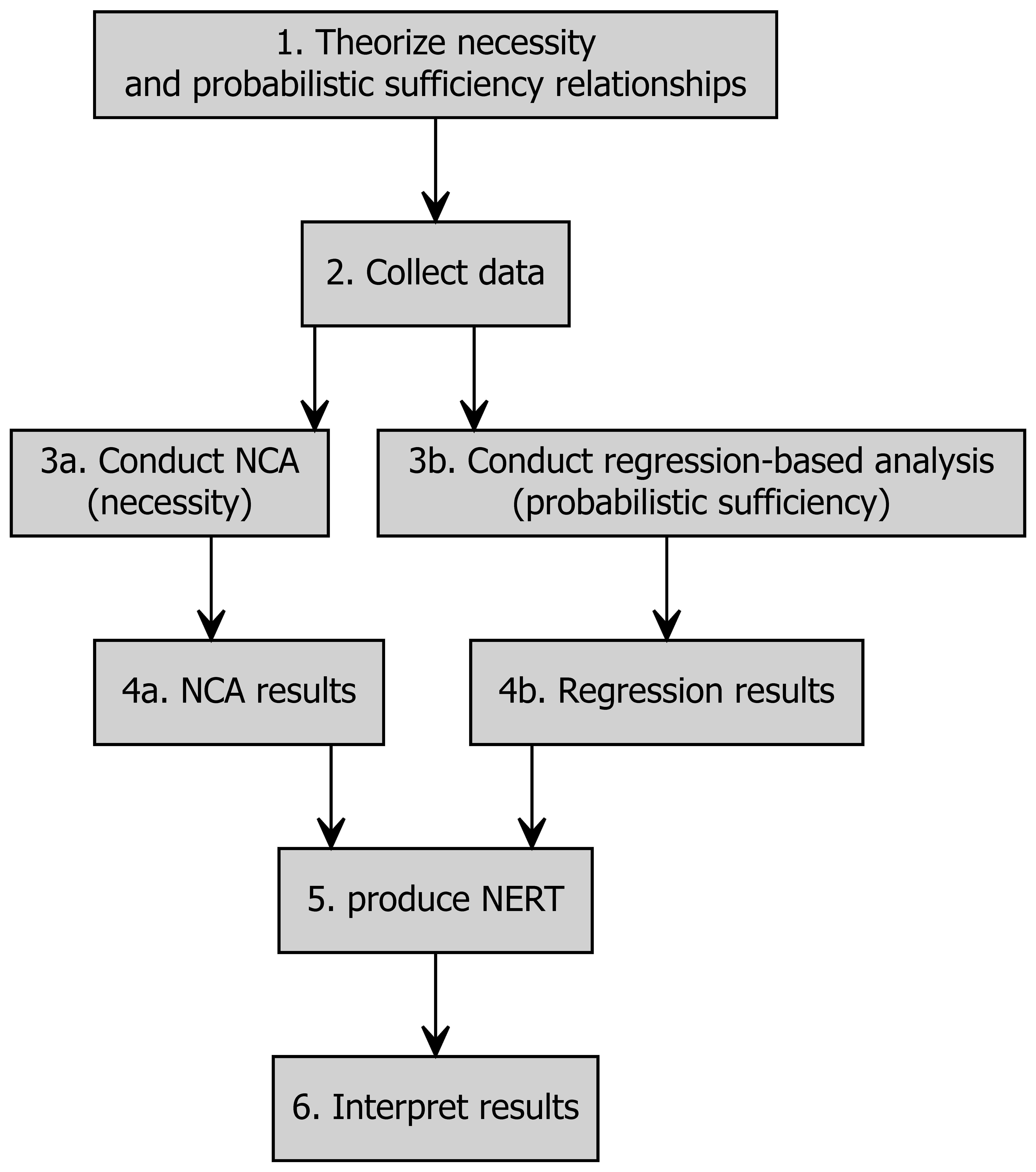
Figure 11.3: Flowchart for conducting a causal pluralism multimethod study with NCA and a regression-based method. NERT = NCA-Extended Regression Table.

The next step is collecting data to obtain valid and reliable scores that represent the \(X\)’s and \(Y\) of the hypotheses (see Chapter 8). Subsequently, two separate data analyses are done: the necessity analysis is conducted with NCA, while the probabilistic sufficiency analysis is done with the selected regression-based analysis (e.g., MLR, SEM). The regression results are often summarized in a regression table that reports the regression coefficients or path coefficients together with their \(p\)-values. Additional information is usually included as well, such as standard errors, confidence intervals, and model fit statistics, and a note may add additional information such as sample size. The left side of Table 11.4 shows a minimum example of such a table with artificial data. In this table the NCA results are added to obtain the NCA-Extended Regression Table (NERT). It expands the conventional regression table by adding two columns: the necessity effect size (\(d\)) and its \(p\)-value, for those predictors that are hypothesized to operate as necessary conditions. A blank line in this table indicates that no theoretical rationale is available, such that the NCA analysis is not conducted for this condition. Additional NCA method information that applies to all tested necessity hypotheses may be added in the note to the table. This applies, for example, to the selected ceiling line for estimating the effect size.

Table 11.4: NERT tool for combining NCA results with regression-based results in a causal-pluralism multimethod study. NERT = NCA-Extended Regression Table. The extension consists of adding two columns to the regression table: the necessity effect size and its \(p\)-value.

	Regression coefficient	p-value	Necessity effect size	p-value
Variables/Conditions
\(X_1\)	0.23	0.035	0.20	< 0.001
\(X_2\)	0.12	< 0.001	0.00	1.000
\(X_3\)	0.43	0.022
\(X_4\)	0.09	0.087	0.03	0.035
\(X_5\)	0.18	0.361	0.12	0.028
Model fit (regression)
\(R^2\) = 0.28
Note:
n = 132. NCA ceiling line: CR-FDH.

A causal-pluralism multimethod study with NCA and a regression-based method can provide complementary information with the following possible results (Table 11.5).

Table 11.5: Possible outcomes of a causal-pluralism multimethod study with NCA and a regression-based method.

	Probabilistic sufficiency If X, then probably Y	Necessity If not X, then not Y
Option 1	Yes	Yes
Option 2	Yes	No
Option 3	No	Yes
Option 4	No	No

• Option 1: \(X\) has an average effect on \(Y\) and is also necessary for \(Y\). \(X\) is not only important but also required for having the outcome (See \(X_1\) in Table 11.4).

• Option 2: \(X\) has an average effect on \(Y\) but is not necessary for \(Y\). \(X\) is important but not essential. Its absence can be compensated by other factors (See \(X_2\) in Table 11.4).

• Option 3: \(X\) has no average effect on \(Y\), but is necessary for \(Y\). It may be that \(X\) is overlooked in regression analysis as an important factor (possibly due to the existence of many cases with high level of \(X\) and low level of \(Y\)), but is still an essential factor. (See \(X_5\) in Table 11.4).

• Option 4: \(X\) has no average effect on \(Y\) and is also not necessary for \(Y\) (See \(X_4\) in Table 11.4).

Note that due to the different causal perspectives, one methodological approach cannot logically be a robustness check of the other approach. The results can only be different, not contradictory.

11.4 Combining NCA and SEM in a multimethod study

One of the most common causal-pluralism multimethod applications of combining NCA with a regression-based method is the use of NCA in the context of structural equation modeling (see Appendices C.3 and C.4). Since in many such published applications NCA is not applied according to the standards proposed in this book and elsewhere, this section (as well as Appendix H) provides more details and recommendations on how to conduct such a combined analysis. A SEM-model consists of two parts. The measurement model defines how specified indicators relate to the underlying constructs (“latent variables”). It determines how the constructs are operationalized by their indicators and how measurement error is represented. The structural model specifies the relationships among the constructs (latent variables). This is the regression-based part of the model.

Different estimation approaches exist for estimating the relationship between the latent variables (“path coefficients”). Conventional covariance-based SEM (CB-SEM, Jöreskog, 1970) estimates model parameters based on the covariance matrix, using techniques such as maximum likelihood. Component-based SEM, for example Partial Least Squares SEM (PLS-SEM, Wold, 1985) estimates latent variable scores as weighted composites of indicators to maximize the explained variance in the dependent variables. A more recent version of PLS is Consistent Partial Least Squares structural equation modeling (PLSc, Dijkstra & Henseler, 2015) that corrects the attenuation bias of traditional PLS estimates when reflective (common-factor) measurement models are used.

If the SEM¹⁰⁴ model is estimated, latent variable scores can be obtained for further analysis, including for use of \(X\)- and \(Y\)-values as input to NCA. In PLS, these scores are directly estimated as part of the model fitting process as component-based SEM-methods are designed to estimate composites, whereas in CB-SEM the analyst must select (based on the analyst’s goals, e.g., unbiasedness, orthogonality, correlation preservation) a factor score estimation method to compute estimated scores for latent factors from observed variables after fitting the model. Thus, depending on the SEM modeling approach that is selected by the analyst, the input scores for NCA and thus the NCA results may differ.

NCA has been applied both in combination with CB-SEM (see Table C.3 in Appendix C.3) and in combination with PLS-SEM (see Table C.4 in Appendix C.4). Using PLS-SEM with NCA is popular, possibly for the following reasons:

1. It is often easier to extract latent variables scores from the estimated PLS models than from estimated CB-SEM models.

2. Leading PLS-SEM proponents introduced NCA as a methodological enrichment of PLS-SEM, and provided specific recommendations (Richter, Schubring, et al., 2020; Richter et al., 2022; Richter, Hauff, Ringle, et al., 2023) and extensions (Hauff et al., 2024; Sarstedt et al., 2024) for combining the methods.

3. A basic version of the NCA software became part of a popular software package originally developed for conducting PLS-SEM (SmartPLS, Section B.4 in the Appendix).

Combining NCA with SEM involves using estimated scores of the latent variables as input for NCA. This allows the analyst to examine whether a relationship between two latent variables is not only related in terms of probabilistic sufficiency (as modeled in SEM) but also in terms of necessity, assuming a theoretical rationale exists. If a formal necessity hypothesis is available or can be derived (see Chapter 7), any pair of latent variables from the structural model can take the role of condition and outcome to study their necessity relationship. When conducting NCA in combination with SEM, all general guidelines for conducting NCA apply (Section 10.3).

The availability of a user-friendly software package for applying NCA within the context of PLS-SEM is an advantage, but it also carries a risk. While the SEM part of the study is often a deductive study for testing a probabilistic sufficiency hypothesis, many published multimethod studies combining NCA and PLS-SEM conduct the NCA part as an exploratory investigation without having a necessity hypothesis. In the absence of a theoretical justification for necessity, such a study cannot claim that necessity has been identified (Section 6.2). This also applies if the theoretical justification is provided after the results are known. An exploratory study does not qualify for a hypothesis testing study (Chapter 7). Having a theoretical rationale before data collection is a prerequisite for making a claim of empirical evidence of necessity (see Section 9.10). After an exploration, a further study is needed to test the hypothesis that was derived from the exploration (Section 7.2).

It is also not uncommon, in particular in studies that combine CB-SEM with NCA, that the latent variable scores of the SEM-part of the study are not used as input to NCA. This happens, for example, when instead of using latent variable scores derived from the SEM study, scores independent from SEM (e.g., means of indicator scores) are used as the latent scores input for NCA. Such a combined NCA-SEM study would qualify as two separate studies according to Table 11.2, as \(X\) and \(Y\) are different in the two studies.

11.4.1 Steps for conducting NCA with SEM

To outline the steps for an NCA-SEM multimethod study, first some SEM terminology is explained. Since SEM terminology about ‘indicators’, ‘weights’, ‘latent variables’ and ‘rescaling’ varies across the SEM literature, the terminology described in Table 11.6 is used in this book.

Table 11.6: SEM terminology

Terms	Description
General
Rescaling	Normalization or standardization of original scores.
Normalization (or min-max normalization)	Rescaling of scales with new minimum and maximum values (e.g., 0–1 or 0–100).
Standardization	Rescaling of observed scale values based on their probability distribution. (z-score: mean = 0 and standard deviation = 1)
Indicator
Indicator (variable)	A manifest/measured variable linked to a latent variable.
Indicator score	The value of an indicator.
Raw indicator score	The value of the indicator measured on its original scale. The scale usually has minimum and maximum values, e.g., Likert scale ranging from 1–5 or 1–7.
Normalized indicator score	The value of an indicator after min-max normalization of the raw indicator score (e.g., 0–1 scale or percentage scale 0–100).
Standardized indicator score	The value of an indicator after standardization of the raw indicator score (z-score).
Original indicator score	The indicator that is used as input for the SEM model, which can be raw or standardized depending on the estimation settings.
Weight and loading
(Indicator) weight	In PLS, the extent to which an indicator contributes to the latent variable score (as part of a weighted composite).
Standardized indicator weight	Indicator weight using standardized indicators.
Estimated indicator weight	In PLS, the estimated coefficient that multiplies an indicator to construct the latent variable score.
Factor loading	The strength of an indicator–latent variable relationship.
Latent variable
Latent variable	An unobserved construct linked to multiple indicators.
Latent variable score	The value of a latent variable, calculated as a linear combination (weighted sum) of indicator scores.
Standardized latent variable score	A weighted linear combination of standardized indicator scores (z-scores). In PLS, these scores are computed directly during model estimation, whereas in CB-SEM they can be derived afterward as estimated factor scores using the model’s factor loadings.
Unstandardized latent variable score	Score obtained as a weighted linear combination of the original (unstandardized) indicator values. In PLS such scores are computed directly; in CB-SEM these scores can be derived post-estimation as factor scores.
Normalized unstandardized latent variable score	Unstandardized latent variable score after normalization.

Figure 11.4 shows a flowchart for conducting NCA in combination with SEM.

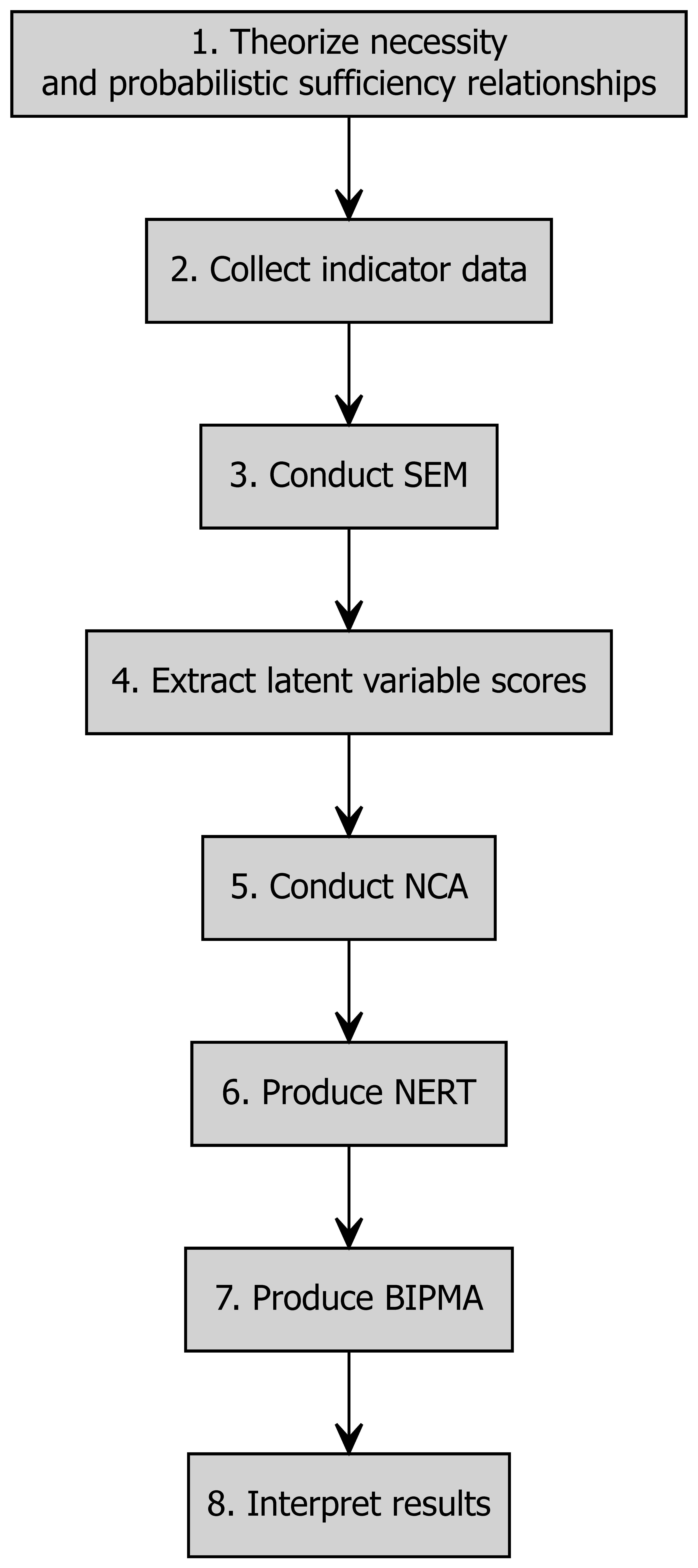
Figure 11.4: Flowchart for conducting NCA in combination with structural equation modeling (SEM). NERT = NCA-Extended Regression Table tool. BIPMA = Bottleneck Importance Performance Map Analysis tool.

Eight steps are distinguished, and each step is discussed in detail. An example is provided in Appendix H.

11.4.1.1 Step 1: Theorize necessity and probabilistic sufficiency

The first step is a fundamental step for any combined NCA and SEM study. An NCA-SEM study implies that the relationships between the variables are considered from two different causal perspectives: necessity (NCA) and probabilistic sufficiency (SEM), see Section 2.7. For inferring causality, both NCA and SEM require that the study starts with formulating theoretical expectations about the causal relationship (e.g., hypotheses). According to SEM, all relationships between latent variables in the structural model are considered probabilistic sufficiency relationships that are theoretically justified. According to NCA, all, a few, or none of these relationships may be hypothesized as necessity relationships as well, depending on the availability of a theoretical justification in the format of a formal necessity hypothesis (Section 7.5). A theory that includes one or more necessity relationships in addition to probabilistic sufficiency relationships is called an ‘embedded necessity theory’ (Bokrantz & Dul, 2023).

Latent variables of a structural model can have different roles. It can be a predictor variable (independent variable; condition in NCA) that has an effect on a predicted variable (dependent variable; outcome in NCA). For example, when in a structural model a latent variable \(M\) mediates the relationship between \(X\) and \(Y\), then \(M\) has two different roles. For the \(X\)-\(M\) relationship \(X\) is the predictor and \(M\) is the predicted variable, and for the \(M\)-\(Y\) relationship \(M\) is the predictor and \(Y\) the predicted variable. When a relationship is (also) considered a necessity relationship, NCA calls the predictor variable the ‘condition’ and the predicted variable the ‘outcome’.

11.4.1.2 Step 2: Collect indicator data

Conducting SEM assumes that data are available on observed indicators. SEM involves specifying a measurement model, which defines the relationships between indicators and latent variables. In step 2 the indicator data are collected. These data are the input for the measurement model.¹⁰⁵

11.4.1.3 Step 3: Conduct SEM

The structural model specifies the relationships between latent variables. The complete model is then estimated using a chosen algorithm (e.g., PLS or CB-SEM). NCA is not part of the SEM estimation process itself, but it uses latent variable scores obtained from SEM as input for its own analysis. Therefore, it is important that the analyst ensures that the latent variable scores extracted from the SEM model are valid, reliable, and interpretable. Recommendations for good SEM practices are available in the literature and are not discussed here. Both commercial and open-source software tools are available to conduct SEM.

11.4.1.4 Step 4: Extract latent variable scores

The latent variable scores obtained from the SEM model serve as input for NCA. During SEM estimation, latent variable scores are often standardized (\(z\)-scores), resulting in scores with a mean of 0 and standard deviation of 1. Although NCA results are invariant to affine transformations (such as standardization or linear rescaling; Section 8.5.2), it is recommended for purposes of interpretation of a necessary condition to first unstandardize standardized latent variable scores. Unstandardized latent variable scores are expressed on a scale that is directly related to the original indicator scale, provided that the same measurement scale was used for all indicators of the latent construct. This allows for more meaningful interpretation of the NCA results, especially when discussing real-world implications and when results are discussed in terms of necessity-in-degree with specified levels of \(X\) and \(Y\). Note that not all SEM software packages offer the option to extract unstandardized latent variable scores. Appendix H gives an example showing how to convert standardized scores back to unstandardized scores when needed.

When all unstandardized latent variable scores are derived from indicators measured on the same scale (i.e., with identical minimum and maximum values), min-max-normalization is not required. However, if latent variables have different scales, min-max normalization is recommended. This ensures that the latent variable scores are comparable, which is particularly important in later steps (e.g., Step 7: producing a BIPMA).

A common approach to min-max normalization is to rescale scores to a 0–100 range, allowing latent variable scores to be interpreted as percentages of their original scale range. Alternatively, rescaling to a 0–1 range can be used, which is often more convenient for NCA, as it yields a scope of 1. However, this is optional and not required for the validity of NCA results.

11.4.1.5 Step 5: Conduct NCA

The unstandardized and possibly min-max normalized latent variable scores are input to NCA. In the first part of the analysis, the hypothesized relationships are tested for necessity-in-kind, which is the qualitative statement that \(X\) is necessary for \(Y\) without specifying levels of \(X\) and \(Y\) other than absence/presence or low/high. The observed effect size \(d\) and the \(p\)-value are compared with their threshold values (e.g., \(d\) = 0.10; \(p\) = 0.05) that are set by the analyst to decide if a predictor variable is necessary for a predicted variable, as suggested by the hypothesis.

In the second part, identified necessary conditions in kind are selected for a bottleneck analysis for necessity-in-degree, which results in a quantitative statement that level \(x\) of \(X\) is necessary for level \(y\) of \(Y\). A specific format of this table, with the outcome values expressed as actual values or percentiles, and the conditions expressed as percentiles, provides information for each latent variable about the percentage of cases that are bottlenecks. A bottleneck case is a case that does not have the required level of the condition for a target level of the outcome.¹⁰⁶

11.4.1.6 Step 6: Produce NERT

The NCA-Extended Regression Table (NERT) summarizes the main SEM results in terms of direct effects (path coefficients), total effects, and their \(p\)-values and the main NCA results in terms of necessity effect sizes and their \(p\)-values. Note again, that NCA is not a robustness check of SEM and vice versa. The two approaches provide different insights due to different causal perspectives.

11.4.1.7 Step 7: Produce BIPMA

Whereas NERT presents the results of both NCA and SEM, the Bottleneck Importance Performance Map Analysis (BIPMA) builds on that by providing a tool to assist practitioners to prioritize their actions and resources based on these results. Evidence-based action means that the action is informed by the results of an empirical study, in particular based on hypotheses that were tested and supported (see the NERT). A SEM-hypothesis is a causal claim about average effects: if \(X\) then probably \(Y\). The hypothesis is usually considered supported if the criteria for statistical significance are satisfied. An NCA-hypothesis is a causal claim about any case: if not \(X\) then not \(Y\). The hypothesis is considered supported if the criteria for statistical significance and for practical significance are satisfied (assuming that a formal necessity hypothesis is available). The NERT reports the effect sizes (total effect for SEM; necessity effect size for NCA) and their significance (\(p\)-values). Only supported hypotheses are considered in BIPMA for evidence-based action.

Taking evidence-based action based only on SEM-results (assuming a supported probabilistic sufficiency hypothesis) means that a predictor variable that has a significant average effect on the predicted variable is a candidate for being changed. The action changes the predictor in order to change the average value of the predicted variable. According to a basic regression assumption, during the change of this predictor all other predictors remain constant (ceteris paribus). This (“all else equal”) assumption is the idea in regression analysis that a coefficient represents the effect of one predictor while holding the other included predictors constant. This implies that only one predictor can be selected for prioritizing an action based on SEM. Selection of multiple predictors and taking action on them simultaneously violates the ceteris paribus requirement. The only evidence-based way to select multiple predictors is through a sequential prioritization, in which a new SEM analysis is conducted after each (hypothetical) change has been made.

A SEM-based action addresses an entire group of cases since SEM results apply to an entire group by definition (average effect). The action is considered most effective if a predictor is “important” and has low “performance.” Importance refers to the strength of the probabilistic sufficiency (average effect) relationship of the predictor variable on the predicted variable. Its metric is the total average effect on the outcome including direct and indirect effects. Performance refers to the mean normalized score of the predictor compared to other predictors. A low performance score means that the predictor has room for improvement. In PLS-SEM, the Importance Performance Map Analysis (IPMA) (Ringle & Sarstedt, 2016) is often used for prioritization. In this map Importance is displayed on the horizontal axis and Performance on the vertical axis. The practical meaning of IPMA is that action priority should be given to a predictor variable with a high level of Importance, and a low level of Performance (points in the bottom-right corner assuming positive total effects and average scores).

Taking evidence-based action based only on NCA results (assuming supported necessity hypotheses) implies that a predictor variable is changed such that a selected target outcome of the predicted variable is possible (though not guaranteed). No assumption is needed about other predictors, including no requirement that these must remain constant. This implies that selection of multiple predictors and taking evidence-based action on them simultaneously is possible. Furthermore, an NCA-based action can address a single case, a small group of cases or an entire group of cases since NCA results apply to all cases. The goal of the action is to ensure that bottleneck cases are resolved: a bottleneck case is a case that does not meet the target condition level that is necessary for the selected target outcome level. An NCA-based action is most effective if only cases are selected that are below the required target condition level (for a detailed discussion see Chapter 12).

In an extension of IPMA, Hauff et al. (2024) introduced the combined Importance Performance Map Analysis (cIPMA) which combines results of NCA and SEM. They add the third dimension that is called here the ‘bottleneck’ dimension. This dimension takes into account how effective the action is from the perspective of the presence of bottleneck cases according to NCA. This means that for cIPMA a target outcome must be selected and that an additional action goal is that the target outcome set by the analyst must become achievable by as many as possible cases. If the target outcome is set at a low level, the goal is to enable a base level of the outcome (e.g., mean or even lower outcome, for example corresponding to a minimum level that is achieved by 50 or 75 percent of the cases). If the target outcome is set at a high level, the goal is to enable high level of the outcome (e.g., corresponding to a minimum level that is achieved by only about 25 or 10 percent of the cases).

NCA’s bottleneck table provides the required information for an NCA-based action in the context of cIPMA. This table is produced in Step 5 of a combined NCA-SEM study (see Figure 11.4). After establishing the target outcome, the bottleneck table provides the corresponding target condition for each necessary condition. The version of the table where conditions are expressed as percentiles provides information about the percentage and the number of cases that are bottleneck cases for the conditions. These cases have not achieved the target condition that is necessary for the target outcome.

The cIPMA plot integrates three dimensions: Importance on the horizontal axis, Performance on the vertical axis, and Bottlenecks represented by the size of the points in the Importance-Performance plot. Each point represents a predictor variable with a given combination of Importance and Performance scores. cIPMA suggests that the best choice is the predictor with the largest Importance score and lowest Performance score (according to SEM), and the largest number of bottleneck cases (according to NCA’s bottleneck table).

When prioritization is based on the combined results from NCA and SEM, only one predictor variable can be selected for change if this change is (also) based on SEM results (because the ceteris paribus assumption of SEM applies). However, it is possible that a bottleneck case is not only a bottleneck for the selected predictor, but also for another predictor. Solving a bottleneck for one predictor (by changing the level of that predictor such that it meets the target condition level) is only effective if the case is not also a bottleneck case for another predictor. A case with multiple bottlenecks (bottlenecks for multiple conditions) remains a bottleneck case after resolving the bottleneck for the selected predictor, because the bottlenecks for the other predictors remain unresolved.

Figure 11.5 shows an example of a Bottleneck Importance Performance Map Analysis (BIPMA).

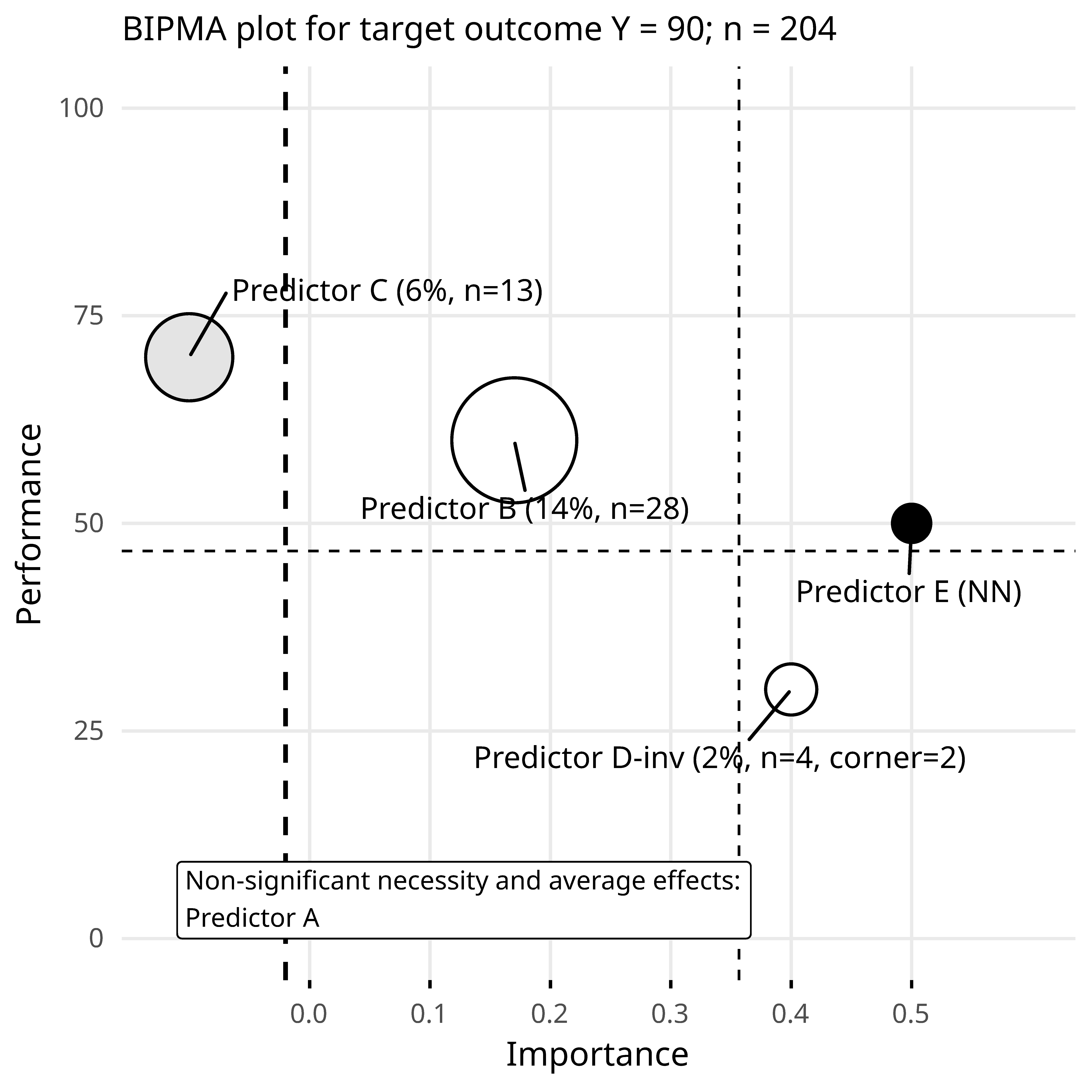
Figure 11.5: Example of a Bottleneck Importance Performance Map Analysis (BIPMA) for evidence-based practical advice (prioritizing predictors) based on NCA and SEM results. The size of the dot is an indication of the number of single bottleneck cases that cannot achieve the target outcome (here 90% of the maximum of the outcome). White points: predictor has a significant necessity effect according to NCA and a significant total average effect according to SEM. Black points: predictor has a non-significant necessity effect and a significant total average effect. Gray points: predictor has a significant necessity effect and a non-significant total average effect. The horizontal and vertical thin dashed lines correspond to mean Performance and the mean Importance of the predictors with a significant total average effect, respectively.

BIPMA differs from cIPMA regarding the bottleneck cases to be considered during prioritization. BIPMA only considers single bottleneck cases. Single bottleneck cases are a bottleneck in only one predictor. These cases are relevant for taking action based on combined results of NCA and SEM. While cIPMA defines the bottleneck dimension for a predictor as the percentage or number of single and multiple bottleneck cases, BIPMA defines it as the percentage or number of single bottleneck cases, only to avoid ineffective actions.

Three additional adaptations compared to cIPMA are implemented in BIPMA. To avoid the risk of false positive conclusions, as a general rule BIPMA only includes predictors to be considered for prioritization when the hypothesis is supported. Although this is a judgment of the analyst, usually an analyst rejects the hypothesis when the \(p\)-value is large (e.g., \(p\ge\) 0.05), suggesting that the observed effect may be compatible with “no effect.”¹⁰⁷ However, cIPMA is asymmetric regarding this statistical significance criterion as it adopts it only for NCA results. cIPMA (and IPMA) allow analysts to consider nonsignificant SEM results for practical action.¹⁰⁸ BIPMA harmonizes this principle by not only excluding non-significant NCA results for evidence-based practical action, but also nonsignificant SEM results. ¹⁰⁹ Since BIPMA is a tool for practical action and not a tool for reporting results of the two analyses, the BIPMA should always be accompanied with the NERT tool (or similar) to report all observed effect sizes and their significance levels.

The second additional adaptation is that BIPMA deals with different relationship directions between predictor variable and predicted variable. The common situation in SEM is that the predictor variable has a positive (average) effect on the predicted variable. BIPMA also handles predictor variables with hypothesized and observed negative total average effects on the predicted variable. For example, Mwesiumo (in press) added a negative total effect for one of the predictor variables on the negative side of cIPMA’s Importance-axis. Since this is inconsistent with the advice (Hauff et al., 2024) that priority should be to points in the bottom-right corner of cIPMA, BIPMA explicitly uses the absolute total effect as Importance score, such that importance scores of positive total effects and negative total effects are comparable and priority should be given to points in the bottom-right corner independent of the sign of the total effect. The BIPMA plot identifies an Importance score that is based on a negative total effect by adding ‘-inv’ to the name of the predictor, indicating that this predictor has an inverse effect on the predicted variable. This is shown in Figure 11.5 for predictor D. While an increase of the predictor variable with a positive total effect will increase the predicted variable, a decrease of the predictor variable with a negative total effect will increase the predicted variable.

A third additional adaptation is that BIPMA also handles different necessity directions. For NCA the default necessity direction is high-high, meaning that a high level of \(X\) is necessary for a high level of \(Y\). The other directions are low-high, high-low, or low-low, suggesting that low \(X\) is necessary for high \(Y\), high \(X\) is necessary for low \(Y\), or low \(X\) is necessary for low \(Y\), respectively. This implies that the expected empty corner of the \(XY\)-plot is not upper-left, but that another corner of the \(XY\)-plot is expected to be empty and should be analyzed. For example, an expected and observed empty corner is the upper-right corner of the \(XY\)-plot (low \(X\) is necessary for high \(Y\)), which implies that for resolving bottleneck cases the predicted variable must decrease, rather than increase. If the corner deviates from corner = 1, the corner is specified in the BIPMA plot in the predictor label. This is shown in Figure 11.5 for predictor D. Predictor D has a negative average effect and an empty upper-right corner in the \(XY\)-plot.

BIPMA aims to inform practice as closely as possible in line with the evidence of empirical results both in terms of effect size and in terms of statistical significance. Using points with different shades of gray, BIPMA displays the four possible combinations of statistical (non-)significance of NCA and SEM results (Figure 11.5):

In BIPMA conditions are displayed as points with different sizes and shades of gray:

• The size of the point reflects the number of single bottleneck cases for the specific condition. The percentage and number of single bottleneck cases is mentioned near the point.

• White point: the total average effect (Importance) and the necessity effect are both significant. The size of the point reflects the number of single bottleneck cases.

• Black point: the total average effect is significant and the necessity effect is non-significant. The black point has a standard size.

• Gray point: the total average effect is non-significant and the necessity effect is significant. The size of the point reflects the number of single bottleneck cases. When according to SEM the average effect of the condition is statistically non-significant only the vertical position (Performance) contains relevant information for action. No evidence-based information is available about the total average effect (Importance). For this reason the point is moved to the left outside the horizontal axis, indicating absence of information.¹¹⁰

• If the total effect is non-significant (statistically) and the necessity effect is non-significant (statistically or practically) the point is not shown. There is no evidence for practical action. The name of such a non-significant predictor is mentioned at the bottom of the plot.

The goal of BIPMA is to identify predictor variables for action using results from NCA and SEM. Several prioritization approaches and corresponding ways to evaluate the BIPMA plot can be used to combine these criteria. Assuming a positive direction for the average effect and a high-high direction for the necessity effect, these strategies can be formulated as follows:

1. Enable a target outcome. This approach only considers NCA results. It is feasible when SEM results do not give a clear preference for predictors to be changed (e.g., no points in the bottom-right corner of BIPMA). Multiple predictor variables can be selected for an action based on the NCA results. This approach implies that the goal of the intervention is to enable a high target score by ensuring that none of the conditions have bottleneck cases. For example, if the target outcome is desirable and \(X\) is necessary for high \(Y\), the target can be set at a high level that is achieved by not more than 25% or 10% of the cases (the level corresponding to the best performing cases). The intervention then consists of ensuring that the bottleneck cases are resolved by increasing the values of the conditions with bottleneck cases. The approach is also feasible when the goal is to enable a certain minimum level of the outcome for all cases. The target outcome can for example be set at a minimum level that is achieved by more than 50% or 75% of the cases.

2. Improve the average outcome. This approach only considers the SEM results. It is feasible when NCA results show that none of the conditions are necessary or there are only a small number of bottleneck cases. Only one predictor variable can be selected for action at once given the ceteris paribus requirement of regression analysis. For selecting a second predictor, evidence-based action requires a new SEM and BIPMA with a new dataset representing the situation after the intervention on the first predictor.

3. Improve the average outcome and enable a target outcome. This approach considers both the NCA and SEM results. Since SEM is part of the consideration, this approach requires that only one predictor is selected for evidence-based action. The combined approach is most effective for a predictor with a large number of bottleneck cases in the bottom-right corner of the BIPMA plot.

Since these stylized situations may not exist in practice, hybrid approaches, for example different approaches for different predictors may be considered.

SEM results are average effect results for the entire group of cases and the goal is to increase the average performance. NCA results allow also custom-made approaches for individual cases or a selection of cases. The case or group of cases gets a specific intervention depending on the case’s bottleneck situation. An individualized NCA-based intervention can considerably improve the intervention effectiveness and efficiency. This is discussed in Chapter 12.

11.4.1.8 Step 8: Interpret results

In the final step the results of the two approaches are interpreted using NERT and BIPMA. It is possible to conduct robustness checks to explore the sensitivity of choices made by the analyst on key results of NCA and SEM. Commonly recommended robustness checks for SEM do not apply to NCA. The NCA-related robustness checks in the context of an NCA-SEM deal with the following two NCA key results that may be affected:

• Identification of a predictor from the SEM structural model as a potential necessary condition.

• Prioritization of predictors for intervention.

As discussed in Section 9.12, these key results may be affected by the analyst’s choices of:

• Ceiling line.

• Threshold level of the effect size.

• Threshold level of the \(p\)-value.

• Scope.

• Outlier handling.

• Target outcome.

A robustness check consists of making an alternative (reasonable) choice rather than the original choice, and studying its influence on the key results. The output of the robustness check is the NCA robustness table. If the influence of changes of the analyst’s choices is small, the original results may be considered robust; if not, the original results may be fragile.

11.4.2 Recommendations for combining NCA and SEM

In publications where NCA is applied in combination with SEM, usually SEM is the main analysis and NCA is used as an additional analysis. However, several guidelines for applying NCA are often violated. This applies, for example, to the following recommendations with ‘must-have’ priority level (see the checklist in Section 10.3):

• Checklist item 4: When, in the context of an NCA study, a comparison is made between NCA’s causal perspective and the causal perspective inferred from conventional regression-based/statistical approaches, use the term probabilistic sufficiency for the latter, and not just sufficiency. The term sufficiency suggests determinism (as applied in QCA’s configurational sufficiency logic). This recommendation is often violated in studies that combine NCA with SEM […].
  See this book: Sections 2.3, 2.4.
  Suggested articles: Dul (2024a) […]
  The results of SEM’s regression analyses (path coefficients of the structural model) are often interpreted as ‘sufficiency’, whereas sufficiency (like necessity) refers to deterministic causal logic and not to the probabilistic causal logic. A better description of the presumed causal relationships of the structural model (like any relationship that is analyzed with regression analysis) would be ‘probabilistic sufficiency’.

• Checklist item 5. In multimethod studies, use and refer to NCA as an approach with a specific perspective on causality and data analysis, and do not incorrectly refer to it as a robustness check or add-on to other methods (and vice versa). This recommendation is often violated in studies that combine NCA with SEM.
  See this book: Sections 2.7, 11.4, 11.5.
  Suggested article: Dul (2024a)
  In studies that combine NCA with SEM, NCA is often suggested as a robustness check of SEM. However, this is incorrect. A good practice is to use NCA as a methodological approach on its own with a different causal perspective, such that the two approaches can give complementary insights.

• Checklist item 7: Formulate the necessity relationship explicitly as a necessary condition hypothesis: \(X\) is necessary for \(Y\). For a deductive study this is done before data analysis; for an explorative study this is done after data analysis when a necessity relationship is found.
  See this book: Sections 7.5.
  In studies that combine NCA with SEM, well-founded probabilistic sufficiency hypotheses are often formulated (to be tested with the SEM model). However, necessity hypotheses are often not provided. Formulating necessity hypotheses is a requirement since the necessity causal perspective differs from the probabilistic sufficiency causal perspective. This applies also to studies that use NCA for exploration or as an additional analysis. A good practice is to formulate necessity hypotheses prior to conducting the analysis, just as is done with the probabilistic sufficiency hypotheses. However, it is estimated that fewer than 25% of NCA-SEM publications include a necessity hypothesis, and a probabilistic sufficiency hypothesis cannot compensate for this absence.

• Checklist item 9: Explain why \(X\) is necessary for \(Y\) using a causal explanation (narrative) by answering three questions: (1) Why does \(X\) enable \(Y\) (\(X\) is an enabler). The existing literature may be a source of information; (2) Why does the absence of \(X\) lead to the absence of \(Y\) (\(X\) is a constraint); (3) Why is the absence of \(X\) not compensable (no substitution for \(X\)). Making the narrative complete is a creative process, supported by literature and experiences of scholars and practitioners.
  See this book: Section 7.5.3.
  This often violated recommendation is related to the previous one. Even if a necessity hypothesis is formulated, it should also be explained why it is expected that \(X\) is necessary for \(Y\) (the causal explanation). Less than half of the few NCA-SEM publications with a necessity hypothesis provide a causal explanation why \(X\) would be necessary for \(Y\). In a theory-testing study, a necessity hypothesis for NCA should get the same attention and depth regarding the causal explanation as a probabilistic sufficiency hypothesis for SEM, as for example is done in a study by Battistoni et al. (2023).

• Checklist item 19: Explain whether and how the data were transformed, and whether the transformation aligns with NCA. Affine transformation (including linear transformation) produces valid results. NCA’s data analysis does not require data transformation and non-transformed data are often more meaningful and better interpretable (e.g., levels of a Likert scale) than transformed data. This particularly applies to necessity-in-degree and interpretations of specific levels of \(X\) being necessary for specific levels of \(Y\). Refrain from conducting non-linear data transformation (e.g., log-transformation, logistic transformation) unless the transformed data represent \(X\) and \(Y\) as defined in the necessity hypothesis (e.g., log-transformed GDP). […].
  See this book: Sections 8.5.2, Appendix D.  
  In most applications of SEM, latent variable scores are standardized (centering the data around zero and scaling the data to have a standard deviation of one). For proper interpretation of necessity-in-degree (bottleneck table) the use of unstandardized scores may be more meaningful. When the indicators are measured on similar scales like Likert scales, unstandardized scores are more closely related to the original measurement scale than standardized scores, which makes interpretations of levels more meaningful.

• Checklist item 20: Specify and justify the selected ceiling line by considering theoretical expectations (border is linear or non-linear), type of data (discrete or continuous), observed border pattern (regular or irregular), balance between accuracy and generalizability (avoiding overfitting), and quality of the data (data with/without measurement error, simulation data).
  See this book: Sections 4.3.2, 9.3.2.   Often no justification is given for the selection of the ceiling line. The CE-FDH ceiling line is commonly selected without further explanation, possibly because this line was used for good reasons in the original publication that introduced NCA in the SEM context (Richter, Schubring, et al., 2020). However, this reason might not apply in other situations. Similarly, when the two default ceiling lines (CE-FDH and CR-FDH) are used, no explanation is usually given for this selection.

• Checklist item 29: Include the \(XY\)-tables or \(XY\)-plots of all tested/explored relationships, preferably in the main text. It is essential that readers are able to inspect them visually.
  See this book: Sections 9.5.
  Often, not all \(XY\)-plots of tested necessity relationships are presented. In some cases, only the plots of the supported relationships are provided. In others, \(XY\)-plots are not provided at all.

• Checklist item 32: Conclude about necessity-in-kind using three criteria: (1) Theoretical justification (the formal hypothesis), (2) Effect size not below the selected threshold value, (3) \(p\)-value below the selected threshold value. Note that for support all criteria apply and that missing just one of them is enough for a rejection. This implies, for example, that without theoretical justification the claim for a necessity relationship is rejected.
  See this book: Sections 9.10.
  In many NCA-SEM studies not all three criteria for concluding about necessity (theoretical support, large effect size, small \(p\)-value) are taken into consideration. Often the requirement of theoretical support is lacking (see items 7 and 9 above). Usually, only theoretical support for the probabilistic sufficiency relationships of the structural model is provided, but this is not informative about the necessity relationship. Without theoretical support for a necessity relationship, it is invalid to conclude that a necessity relationship was identified, even if the effect size was large enough, and the \(p\)-value small enough.

• Checklist item 36: Conduct robustness checks and summarize the results: is the main conclusion about necessity (support or rejection of the hypothesis) sensitive to choices by the analyst regarding ceiling line, scope, effect size threshold, \(p\)-value threshold, removing/keeping outliers, different choices for the target outcome? Conclude if the results are robust or fragile.
  See this book: Section 9.12.
  In many studies a robustness check is done for the SEM part of the study, but not for the NCA part. Robustness checks for NCA are different from those for SEM, and equally important. For example, outliers for SEM may not be outliers for NCA, and vice versa. NCA’s outlier analysis can be done with the NCA software in R (Section H.8 in the Appendix H for an example).

• Checklist item 38: When NCA is used in a causal-pluralism study by combining it with another method (e.g., regression-based methods or QCA), report how the results of NCA and the other method complement each other using NERT, NEST and BIPMA when applicable.
  See this book: Chapter 11.
  In many studies, SEM results and NCA results are presented separately without discussing the insights obtained from combining the two methods. The discussion could focus on the consequences of the combined results for theory and practice. The use of NERT (Section 11.3) and BIPMA (Section 11.4.1.7) could be helpful to integrate the results.

The quality of studies that combine NCA with SEM could be enhanced by ensuring that these and other ‘must-have’ recommendations are fulfilled. Once the must-have requirements are met, further improvements can be achieved by addressing the ‘should-have’ and ‘nice-to-have’ suggestions in the checklist (Section 10.3). As the number of combined NCA and SEM studies grows, reviewers may raise the standard for the appropriate application of NCA. Section 10.3 includes recommendations and references to meet the requirements.

Appendix H provides a demonstration of combining NCA and PLS-SEM with R.

11.5 NCA with QCA

Qualitative Comparative Analysis (QCA) has its roots in political science and sociology, and was developed by Charles Ragin (Ragin, 1987, 2000, 2008). QCA has steadily evolved over the years, and currently many types of QCA approaches exist. A common interpretation of QCA as described by Schneider & Wagemann (2012) and Mello (2021) is followed in this book.

11.5.1 Principles of QCA

Set theory is at the core of QCA. Instead of studying relations between variables, set theory focuses on relations between sets. Cases can be either part of a set or not part of a set. The Netherlands, for example, is a case that is ‘in the set’ of rich countries, and Ethiopia is a case that is ‘out of the set’ of rich countries. Set membership scores (rather than variable scores) are linked to a case. Regarding the set of rich countries, the Netherlands has a set membership score of 1 and Ethiopia of 0. In the original version of QCA the set membership scores could only be 0 or 1. This version of QCA is called crisp-set QCA (csQCA). Later also fuzzy-set QCA (fsQCA) was developed. Here the membership scores can also have values between 0 and 1. For example, Croatia could be allocated a set membership score of 0.7, indicating that it is ‘more in the set’ than ‘out of the set’ of rich countries.

In QCA, relations between sets are studied. Suppose that one set is the set of rich countries (\(X\)), and another set is the set of countries with happy people (‘happy countries’, \(Y\)). QCA uses Boolean (binary) algebra and expresses the relationship between condition \(X\) and outcome \(Y\): the presence or absence of \(X\) is related to the presence or absence of \(Y\). More specifically, the relations are expressed in terms of sufficiency and necessity. For example, the presence of \(X\) (being a country that is part of the set of rich countries) could be theoretically stated as sufficient for the presence of \(Y\) (being a country that is part of the set of happy countries). In this case, the following claims would apply: All rich countries are happy countries; the set of rich countries is a subset of the set of happy countries; no rich country is not a happy country; set \(X\) is a subset of set \(Y\). Alternatively, another theory could state that the presence of \(X\) (being a country that is part of the set of rich countries) is necessary for the presence of \(Y\) (being a country that is part of the set of happy countries). All happy countries are rich countries; the set of rich countries is a superset of the set of happy countries; no happy country is not a rich country; set \(X\) is a superset of set \(Y\).

QCA’s main causal interest is sufficiency. QCA assumes that a configuration of single conditions produces the outcome. For example, the condition of being in the set of rich countries (\(X_1\)) AND the condition of being in the set of democratic countries (\(X_2\)) is sufficient for the outcome of being in the set of happy countries (\(Y\)). QCA’s Boolean logic statements for this sufficiency relationship is expressed as follows:

\[\begin{equation} \tag{11.2} X_1*X_2 → Y \end{equation}\]

where the symbol ‘\(*\)’ means the logical ‘AND’, and the symbol ‘\(→\)’ means ‘is sufficient for’.

Furthermore, QCA assumes that several alternative configurations may exist that can produce the outcome, known as ‘equifinality’. This is expressed in the following example:

\[\begin{equation} \tag{11.3} X_1*X_2 + X_2*X_3*X_4 → Y \end{equation}\]

where the symbol ‘\(+\)’ means the logical ‘OR’.

It is also possible that the absence of a condition is part of a configuration. This is shown in the following example:

\[\begin{equation} \tag{11.4} X_1*X_2 + X_2*{\neg}X_3*X_4 → Y \end{equation}\]

where the symbol ‘\(\neg\)’ means ‘absence of’.

Single conditions that are necessary/non-redundant in a configuration that is sufficient for the outcome are called INUS conditions (Mackie, 1965). An INUS condition is an ‘Insufficient but Non-redundant (i.e., Necessary) part of an Unnecessary but Sufficient condition.’ In this expression, the words ‘part’ and ‘condition’ are somewhat confusing because ‘part’ refers to the single condition and ‘condition’ refers to the configuration that consists of single conditions (parts). Insufficient refers to the fact that a part (single condition) is not itself sufficient for the outcome. Non-redundant refers to the necessity of the part (single condition) for the configurations being sufficient for the outcome. Unnecessary refers to the possibility that other configurations can also be sufficient for the outcome. Sufficient refers to the fact that the configuration is sufficient for the outcome.

Although a single condition may be locally necessary for the configuration to be sufficient to produce the outcome, it is not globally necessary for the outcome because the single condition may be absent in another sufficient configuration. INUS conditions are thus usually not necessary conditions for the outcome (the latter are the conditions that NCA considers). Hence, in above generic logical statements about relations between sets, see Equations (11.2), (11.3), (11.4), \(X\) and \(Y\) can only be absent or present (Boolean algebra), even though the individual members of the sets can have fuzzy scores. Both csQCA and fsQCA use only binary levels (absent or present) of the condition and the outcome when formulating the solution.

The starting point of QCA’s data analysis is to transform variable scores (if available) into set membership scores. Variable scores are called “raw” scores and the transformation process is called ‘calibration’. Calibration can be based on the distribution of the data, the measurement scale, or expert knowledge. The goal of calibration is to get scores of 0 or 1 (csQCA) or between 0 and 1 (fsQCA) to represent the extent to which the case belongs to the set (set membership score). In fsQCA, cases with membership score below 0.5 do not count as having the condition present and contribute to the assessment of absence of the condition. Similarly, cases with membership score above 0.5 qualify as having the condition present.

As a qualitative method, QCA’s calibration process is preferably guided by knowledge about the studied cases. However, particularly in large-n fsQCA studies a ‘mechanistic’ (data driven) transformation is often unavoidable due to lack of access to the cases. For this transformation the non-linear logistic function is usually selected. This selection is somewhat arbitrary (but is built into popular QCA software) and moves the variable scores to the extremes (0 and 1) in comparison to just (linear) transformation (e.g., min-max normalization) of the data. With the standard logistic transformation, low values move toward 0 and high values toward 1. When no substantive reason exists for the logistic transformation, and mechanistic transformation is unavoidable, linear transformation from raw scores to set membership scores (normalization) may be preferred to avoid changing the distribution of the data and obscure possible necessary conditions (Dul, 2016b). Moving the \(X\)- and \(Y\)-scores to the extremes implies that cases in the \(XY\)-plot with low to middle values of \(X\) move to the left and cases with middle to high values of \(Y\) move upwards. As a result, the upper-left corner is filled with more cases. Consequently, potential meaningful empty spaces in the original data (indicating necessity) may not be identifiable. With the normalized transformation, the cases stay where they are; an empty space in a corner of the \(XY\)-plot with the original data stays empty. The normalized transformation is an alternative to an arbitrary transformation: it just changes variable scores into set membership scores, without affecting the distribution of the data. A calibration evaluation tool to check the effect of calibration on the necessity effect size is available at https://r.erim.eur.nl/r-apps/qca/.

QCA performs two separate analyses with calibrated data: a necessity analysis for identifying necessary conditions¹¹¹, and a sufficiency analysis (‘truth table’ analysis) for identifying sufficient configurations. Although the focus in QCA is on sufficiency, a necessity analysis precedes the sufficiency analysis because if a necessary condition is not part of the sufficient configuration, the outcome will not be produced:

“If a causal condition passes the analyst’s test of necessity, then this condition should be made a component of every causal expression that the analyst examines subsequently in the analysis of sufficiency” (Ragin, 2000, p. 254)

In csQCA, \(X\) and \(Y\) are expressed as dichotomous set membership scores: present (in the set) or absent (not in the set). In the \(XY\)-table, a necessary condition in kind is identified when the upper-left cell is (almost) empty (Figure 11.6). Necessity consistency is the number of cases in the upper-right cell divided by the number of cases in the upper-left plus upper-right cell.

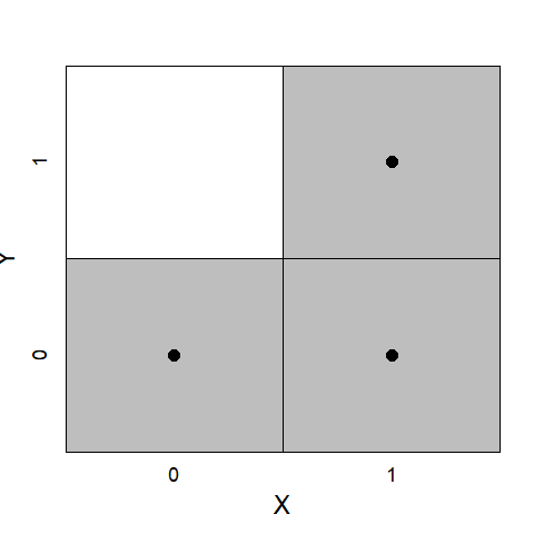
Figure 11.6: Necessity analysis by dichotomous NCA and crisp set QCA.

In fsQCA, \(X\) and \(Y\) are expressed as discrete or continuous set membership scores indicating the extent to which the condition or outcome is in the set. In the \(XY\)-plot, a diagonal is drawn and a necessary condition in kind is identified when the area above the diagonal is (almost) empty (Figure 11.7-left). Necessity inconsistency is the sum of vertical distances of cases above the diagonal, divided by the sum of vertical distances of all cases. Necessity consistency is the complement of this value (1 − inconsistency).

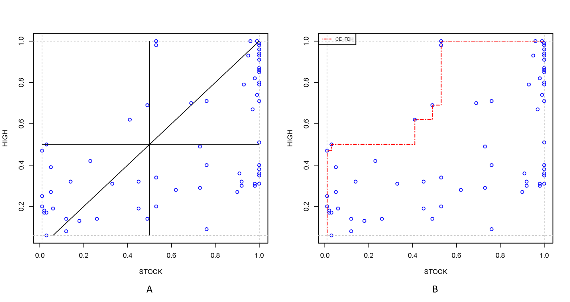
Figure 11.7: Comparison of necessity analysis with fsQCA (Left) and with NCA (Right). The ceiling in QCA is predefined (diagonal) and in NCA estimated (with CE-FDH). Data from Rohlfing & Schneider (2013); see also Vis & Dul (2018).

The main analysis of csQCA and fsQCA is the sufficiency analysis. Whereas QCA’s necessity analysis uses linear algebra to identify necessity, QCA’s sufficiency analysis uses Boolean algebra and truth tables. The truth table is a logical summary of all (\(2^k\)) possible combinations of \(k\) conditions (\(X\)’s) that are selected for the analysis. A combination of conditions is referred to as a configuration. In configurations, conditions can only be considered present or absent (with the 0.5 membership score threshold point used in fsQCA; absent: < 0.5; present: > 0.5). The purpose of QCA is to identify which of the possible configurations in the truth table are actually observed in the data, and to establish whether the outcome is present or absent in the observed configurations. This leads to QCA’s solution table consisting of configurations that are considered to be able to produce the outcome (\(Y\) = 1). A second solution table consists of configurations that are considered to not produce the outcome (\(Y\) = 0).

Over the years, different approaches have been suggested to integrate an observed necessary condition from QCA’s necessity analysis (for \(Y\) = 1 and \(Y\) = 0, respectively) into the sufficiency solution. For example, Ragin has suggested to add the necessary condition if it is absent in an observed configuration, to remove the necessary condition from all configurations, and to ignore necessity.¹¹² It appears that the necessity analysis of QCA is often ignored and if this analysis is done, different approaches are used for integration of the necessity analysis with the sufficiency analysis.

11.5.2 Comparison NCA and QCA

NCA and QCA share several characteristics. For a causal interpretation of data, both NCA and QCA rely on conditional logic (necessity and sufficiency), and theoretical argumentation for causality. Although NCA primarily uses quantitative variable-based approaches, it can also be applied (like QCA) with calibrated set membership scores. Both methods can be used in large-n or small-n settings. In a large-n setting, both methods preferably use probability sampling and statistical generalization, although this is not common in QCA (Braumoeller, 2015).

Despite these similarities there are also major differences (Dul, 2016a; Vis & Dul, 2018). NCA focuses on necessity, whereas QCA focuses on sufficiency. NCA is mainly a deductive approach requiring a formal necessity hypothesis whereas QCA is mainly an inductive approach. Although QCA carefully selects conditions, a hypothesis how these are related to the outcome is usually not provided. The difference is evident when analyzing OR-combinations of necessity. An OR-combination (\(X_1\) or \(X_2\) is necessary for \(Y\)) is often an indication that a higher order construct is necessary for the outcome. A green apple is not necessary for an apple pie, nor is a red apple, but apple is necessary for an apple pie. In NCA’s procedures for formulating a formal necessary condition hypothesis (Chapter 7), a relevant higher order construct, rather than the related lower order construct, would likely be recognized and become part of the analysis. An inductive QCA approach may not consider OR-combinations before the analysis, but may identify them afterwards. However, many identified necessity OR-combinations have no substantive meaning as by logic, any necessary condition that is combined with another condition is a necessary OR-combination, even if the combination does not have a substantive meaning. If apple is necessary for an apple pie, then the combination [apple OR blue sky] is also necessary by logic, but this does not mean that blue sky is necessary or relevant. The combination is logically true but substantively meaningless.

Since NCA is an approach for analyzing necessity, it can be compared with QCA’s necessity analysis only. When NCA is applied with dichotomous set membership scores as input for NCA’s necessity analysis, the conclusions are usually the same as with csQCA’s necessity analysis. Without cases in the upper-left cell, QCA’s consistency = 1, which supports necessity. In this situation NCA’s effect size is 1, and assuming theoretical support and statistical significance, NCA supports necessity as well. However, NCA differs completely from fsQCA’s necessity analysis. Whereas in fsQCA the ‘ceiling line’ is predefined as the diagonal in the \(XY\)-plot (Figure 11.7-left), in NCA the ceiling line is usually estimated from data¹¹³, which is usually above the diagonal. When fsQCA rejects necessity when too many cases are above the diagonal (using necessity consistency as model fit measure), NCA’s necessity analysis may conclude that necessity does exist, though not for all levels of \(X\) and \(Y\). Whether or not necessity-in-kind should be rejected depends in NCA on the effect size, the availability of theoretical support for necessity and the \(p\)-value (Section 9.10), but not directly on its model fit measures (Section 4.5). Additionally, when necessity-in-kind is observed, NCA can analyze necessity-in-degree to evaluate which level of \(X\) is necessary for which level of \(Y\) (Section 9.11).

When fsQCA supports necessity, some cases may be in the ‘empty’ zone above the diagonal as deviant cases. According to NCA the same cases may be close to but below the ceiling line and may be considered best cases: cases that are able to achieve a high outcome with a low level of the conditions (assuming that \(X\) is an effort and \(Y\) is a desired outcome). In NCA, cases above the ceiling are considered not feasible and classified as noise (close above to the ceiling) or outliers/exceptions (further away from the ceiling) as discussed in Section 4.5.

11.5.3 Combining NCA and QCA

There are two ways to combine NCA and QCA in a multimethod study. First, since both NCA and QCA employ a necessity analysis based on necessity causal logic, these two approaches can be used jointly in a method-triangulation multimethod study. Second, since QCA also employs a sufficiency analysis based on configurational sufficiency causal logic, NCA can be combined with QCA’s sufficiency analysis in a causal-pluralism multimethod study. Both types of multimethod studies are discussed below in more detail.

11.6 Combining NCA and QCA in a multimethod study

11.6.1 Steps for conducting NCA with QCA’s necessity analysis

Figure 11.8 shows a flowchart for conducting a necessity analysis with NCA and QCA in a method-triangulation multimethod study.

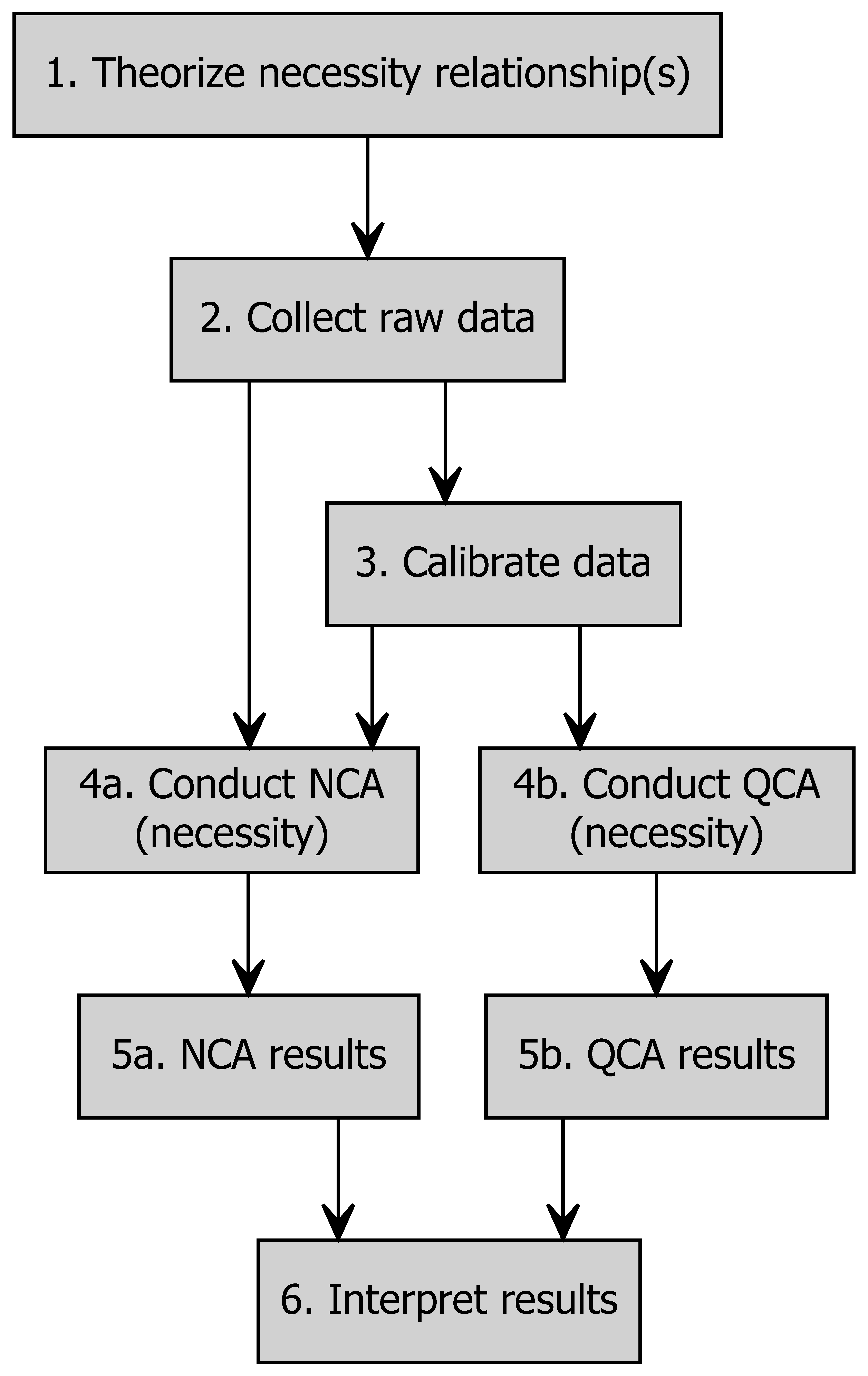
Figure 11.8: Flowchart for conducting a method-triangulation multimethod study with NCA and QCA’s necessity analysis.

The study starts with theorizing the necessity relationship(s). In NCA this means the formulation of a formal necessity hypothesis (Chapter 7) in which not only \(X\) and \(Y\) are selected, but also the causal relationship is theoretically justified. In QCA the relationship between the conditions and outcome is usually not discussed extensively before the analysis is done and usually no necessity hypothesis is formulated. This reflects that QCA is a more inductive approach.

The next step is collecting (raw) data. In QCA the data need to be calibrated to transform the data into meaningful set membership scores. Qualitative data may be calibrated based on case knowledge of the user and expert judgment (the direct method), and quantitative data can be calibrated by mechanistically applying a transformation function (the indirect method). NCA accepts both calibrated data and raw data (when the raw data are valid and reliable), but QCA accepts only calibrated data. Therefore, two types of NCA-QCA method-triangulation for analyzing necessity can be done:

1. NCA with raw data and QCA with calibrated data.

2. NCA and QCA both with calibrated data.

After the NCA and QCA analyses are conducted, in the last step the results are interpreted in combination.

11.6.2 Example NCA-QCA method-triangulation multimethod study

This section presents an example of integrating NCA in QCA according to a method-triangulation multimethod necessity study. The example is based on a study by Lipset (1959), discussed in Ragin (2009). The outcome variable is SURV: survival of democracy during the inter-war period. Assuming that a theoretical rationale for necessity exists, five conditions were analyzed for necessity using both QCA and NCA:

• DEV: Level of development: expressed as GDP per capita (USD) in the raw data.

• URB Level of urbanization: percent of the population in towns with 20,000 or more inhabitants in the raw data.

• LIT Level of literacy: percent of the literate population (raw data).

• IND Level of industrialization: percent of the industrial labor force (raw data).

• STB Government stability: “political-institutional (in)stability” expressed in the raw data by the number of cabinets which governed in the period under study.

The raw data were calibrated into fuzzy set membership scores (the calibration process is not discussed here). The analyses can be done as follows:

library(QCA)
library(NCA)

# Data
conditions <- c("DEV", "URB", "LIT", "IND", "STB") #names of the conditions
outcome <- "SURV" #name of the outcome
data(LR) #Lipset raw data
data(LF) #Lipset calibrated data

#QCA-calibrated (fuzzy)
pofind(LF, outcome = "SURV") #single necessary conditions

## 
##            inclN   RoN   covN  
## ------------------------------ 
##  1   ~DEV  0.285  0.587  0.274 
##  2    DEV  0.831  0.811  0.775 
##  3   ~URB  0.568  0.452  0.402 
##  4    URB  0.539  0.899  0.771 
##  5   ~LIT  0.096  0.764  0.168 
##  6    LIT  0.991  0.509  0.643 
##  7   ~IND  0.417  0.576  0.367 
##  8    IND  0.669  0.786  0.684 
##  9   ~STB  0.218  0.687  0.269 
## 10    STB  0.920  0.680  0.707 
## ------------------------------

#NCA-calibrated (fuzzy)
set.seed(123) # for reproducible results
model_calibrated<- nca_analysis(LF,
                                1:5,6,
                                ceilings = "ce_fdh",
                                test.rep = 10000)

## Setting up parallelization, this might take a few seconds...                                                               Do test for  :  ce_fdh - DEVDone test for:  ce_fdh - DEV       
## Do test for  :  ce_fdh - URBDone test for:  ce_fdh - URB       
## Do test for  :  ce_fdh - LITDone test for:  ce_fdh - LIT       
## Do test for  :  ce_fdh - INDDone test for:  ce_fdh - IND       
## Do test for  :  ce_fdh - STBDone test for:  ce_fdh - STB

model_calibrated

## 
## ---------------------------------------------------------------------------

## Effect size(s):

##     ce_fdh p    
## DEV 0.37   0.000
## URB 0.01   0.359
## LIT 0.82   0.002
## IND 0.02   0.359
## STB 0.46   0.004
## ---------------------------------------------------------------------------

# NCA-raw data
set.seed(123) # for reproducible results
model_raw <- nca_analysis(LR,
                          1:5,6,
                          ceilings = "ce_fdh",
                          corner = c(1,1,1,1,2),
                          test.rep = 10000)

## Setting up parallelization, this might take a few seconds...                                                               Do test for  :  ce_fdh - DEVDone test for:  ce_fdh - DEV       
## Do test for  :  ce_fdh - URBDone test for:  ce_fdh - URB       
## Do test for  :  ce_fdh - LITDone test for:  ce_fdh - LIT       
## Do test for  :  ce_fdh - INDDone test for:  ce_fdh - IND       
## Do test for  :  ce_fdh - STBDone test for:  ce_fdh - STB

model_raw

## 
## ---------------------------------------------------------------------------

## Effect size(s):

##     ce_fdh p    
## DEV 0.27   0.000
## URB 0.09   0.339
## LIT 0.74   0.001
## IND 0.11   0.095
## STB 0.53   0.010
## ---------------------------------------------------------------------------

Table 11.7 shows the results. Using the common necessity consistency threshold of 0.9 two necessary conditions are identified by QCA: LIT and STB. NCA’s necessity analysis with the raw and with calibrated data show similar results. Also, NCA shows that LIT and STB are necessary conditions. However, NCA identifies a third necessary condition: DEV.

Table 11.7: Comparison of NCA’s and QCA’s necessity analyses in a method-triangulation multimethod study.

	QCA Consistency (calibrated)	Necessity effect size (calibrated)	p-value (calibrated)	Necessity effect size (raw)	p-value (raw)
\(DEV\)	0.831	0.37	< 0.001	0.27	< 0.001
\(URB\)	0.539	0.01	0.361	0.09	0.336
\(LIT\)	0.991	0.82	0.002	0.74	0.001
\(IND\)	0.669	0.02	0.366	0.11	0.097
\(STB\)	0.920	0.46	0.004	0.53	0.008

Generally, NCA identifies more necessary conditions than fsQCA. This particularly happens when raw data, rather than (mechanistically) calibrated data, are used as input to NCA. For example, Torres & Godinho (2022) conducted a method-triangulation NCA-QCA necessity study. They examined which elements of digital entrepreneurial ecosystems are necessary to produce outcomes. In their study the authors used only calibrated data and concluded that “[…] fsQCA should be complemented with NCA to better understand the necessary conditions. The results show that the former identifies considerably less necessary conditions in data sets than NCA[…]” (Torres & Godinho, 2022, p. 41).

11.6.3 Steps for conducting NCA with QCA’s sufficiency analysis

Another type of NCA-QCA multimethod study is the causal-pluralism multimethod study in which NCA’s necessity causal perspective is combined with QCA’s configurational sufficiency causal perspective. For a causal-pluralism study, it is necessary that the two methods use the same data. Hence, NCA must be applied with set membership scores, otherwise comparing and combining necessity results with sufficiency results becomes problematic.¹¹⁴

Figure 11.9 shows a flowchart for conducting a necessity analysis of NCA with a sufficiency analysis of QCA in a causal-pluralism multimethod study.

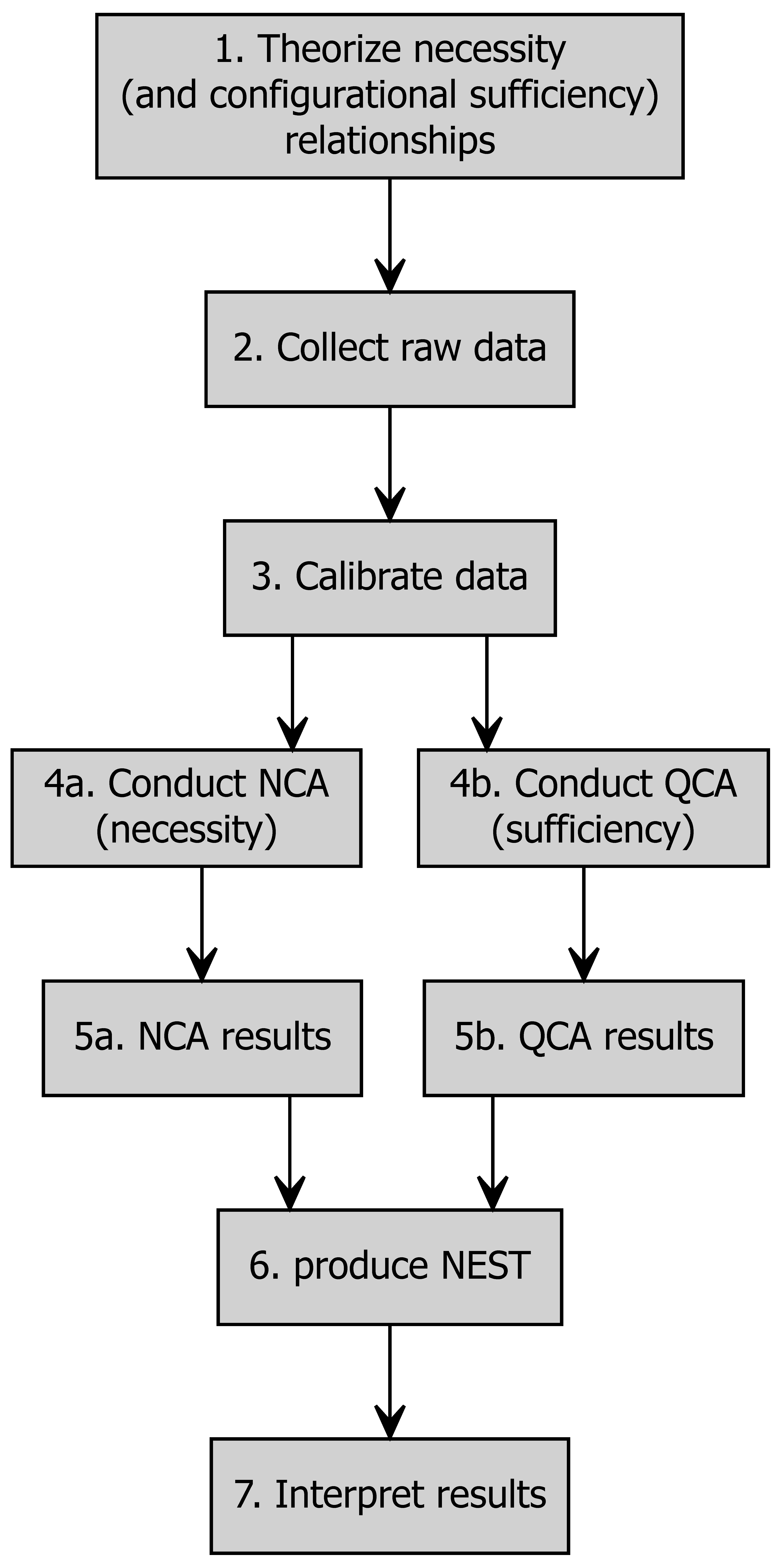
Figure 11.9: Flowchart for conducting a causal-pluralism multimethod study with NCA and QCA’s sufficiency analysis.

The study starts with theorizing the necessity relationships for NCA: the formulation of a formal necessity hypothesis (Chapter 7). For the QCA sufficiency analysis the conditions that are part of the necessity hypothesis, and possibly other non-necessary contributing conditions are selected. Often, QCA is used inductively and does not formulate sufficiency hypotheses (claims about configurations that can produce the outcome) although this is also possible as, for example, suggested by Mello (2021). Next, the raw data are collected and subsequently calibrated. The set membership scores are input to both NCA and QCA. Then NCA and QCA are conducted according to their own standards.

After the two analyses are done, the integration of the results may be challenging. As indicated in the above quote by Ragin, a necessary condition must become a part of the sufficient configuration, otherwise the configuration will not produce the outcome. Ragin’s views on how to realize that goal has changed over the years, and new views have been added. Currently, at least five different views exist in the QCA community on how to integrate the identified necessary conditions (with QCA) with the identified sufficient configurations. These views may also apply to integrating a necessary condition identified with NCA.

In the first view, only sufficient configurations that include the necessary conditions are considered. This ensures that all selected configurations have the necessary condition. In the second view, the truth table analysis to find the sufficient configurations is done without the necessary conditions, and afterwards the necessary conditions are added to the configuration. This also ensures that all configurations have the necessary conditions. In the third view, configurations that do not include the necessary condition are excluded from the truth table before this table is further analyzed to find the sufficient configurations. This ‘ESA’ approach (Schneider & Wagemann, 2012) also ensures that all configurations have the necessary conditions. In the fourth view, sufficient configurations are analyzed without worrying about necessary conditions. Afterwards, the necessary conditions are discussed separately. In the fifth view, a separate necessity analysis is not done, or necessity is ignored.

All views have been employed in QCA; no consensus exists yet. An additional complexity of integrating NCA’s necessity with QCA’s sufficient configurations is that NCA produces necessary conditions in degree, rather than QCA’s necessary conditions in kind. In QCA’s solution table, the conditions that are part of the sufficient configurations can only be absent or present.

One way to proceed with integrating NCA ’s necessity approach with QCA’s sufficiency approach is to combine the last part of the second view (adding necessary conditions afterwards), with the fourth view (discussing necessary conditions separately):

1. After NCA has identified necessity-in-kind in step 4a and QCA has identified the solution table in step 4b, NCA’s bottleneck analysis for necessity-in-degree is conducted in step 5a, NCA’s necessity-in-degree analysis with the bottleneck table is conducted as follows. Since in QCA’s solution table an outcome is considered to be in the set if the set membership score is \(Y\) > 0.5, NCA’s necessity-in-degree analysis consists of identifying the required level of the condition membership score \(X\) that is necessary for an outcome membership score \(Y\) of at least 0.5. In other words, the target outcome in the bottleneck table is \(Y\) = 0.5 membership score.

2. Next, the resulting required membership score of the condition according to NCA is added to all QCA’s sufficient configurations in the solution table, if this condition is not already part of the configuration. Specifically, the NCA-Extended Solution Table (NEST) is produced. This extension specifies the required level of the necessary condition identified by NCA, such that the configuration can produce the outcome (for an example see below).

3. Finally, the result of the NEST and the full results of NCA’s necessity analysis and QCA’s sufficiency analysis are interpreted in combination. In particular, it could be discussed that specific levels of necessary membership scores found by NCA must be present in each sufficient configuration found by QCA. If that membership in degree is not in place, the configuration will not produce the outcome.

11.6.4 Example NCA-QCA causal-pluralism multimethod study

This section presents an example of integrating NCA in QCA according to a causal-pluralism multimethod necessity-sufficiency study. The example is based on a study by Emmenegger (2011) about job security regulation (JSR) in Western European countries. In particular, the effect of six conditions is investigated. These six conditions are: S = state-society relationships, C = non-market coordination, L = strength labor movement, R = denomination, P = strength religious parties and V = veto points. The study conducts a necessity analysis and a sufficiency analysis, both with fsQCA. The study can be replicated as follows:

library(QCA)

# Data
data("d.Emm")
conditions <- c("S","C","L","R","P","V") #names of the conditions
outcome <- "JSR" #name of the outcome

##### QCA #####
pofind(d.Emm, outcome = "JSR") #single necessary conditions

## 
##          inclN   RoN   covN  
## ---------------------------- 
##  1   ~S  0.438  0.639  0.453 
##  2    S  0.667  0.783  0.714 
##  3   ~C  0.543  0.615  0.509 
##  4    C  0.620  0.833  0.743 
##  5   ~L  0.571  0.677  0.571 
##  6    L  0.714  0.843  0.793 
##  7   ~R  0.388  0.661  0.431 
##  8    R  0.791  0.812  0.791 
##  9   ~P  0.528  0.612  0.498 
## 10    P  0.672  0.863  0.800 
## 11   ~V  0.648  0.692  0.627 
## 12    V  0.500  0.738  0.577 
## ----------------------------

#published solution: no necessary conditions with consistency > 0.9
ttEmm <- truthTable(d.Emm, condition =  conditions,
                     outcome = outcome,
                     incl.cut = 0.90,
                     show.cases = TRUE)

# conservative/complex solution
minimize(ttEmm) 

## 
## M1: S*~C*L*R*P + S*C*R*P*V + S*~C*~L*R*~P*~V + ~S*C*L*~R*P*~V -> JSR

#M1: S*~C*L*R*P + S*C*R*P*V + S*~C*~L*R*~P*~V + ~S*C*L*~R*P*~V -> JSR

# parsimonious solution
minimize(ttEmm, include =  "?") 

## 
## M1: S*R + (L*P) -> JSR 
## M2: S*R + (P*~V) -> JSR

#M1: S*R + (L*P) -> JSR
#M2: S*R + (P*~V) -> JSR

# intermediate solution
minimize(ttEmm, include = "?", dir.exp = c(1,1,1,1,1,0), details=T)

## 
## From C1P1, C1P2: 
## 
## M1:    S*R*~V + S*C*R*P + S*L*R*P + C*L*P*~V -> JSR 
## 
##              inclS   PRI   covS   covU   cases 
## --------------------------------------------------- 
## 1    S*R*~V  0.990  0.983  0.402  0.152  FR,PT; IT 
## 2   S*C*R*P  0.965  0.921  0.277  0.041  BE,DE; AT 
## 3   S*L*R*P  1.000  1.000  0.354  0.027  IT; ES; AT 
## 4  C*L*P*~V  0.964  0.872  0.297  0.138  NO 
## --------------------------------------------------- 
##          M1  0.965  0.941  0.685

#M1:    S*R*~V + S*C*R*P + S*L*R*P + C*L*P*~V -> JSR

#published solution: 
#M1:    S*R*~V + S*C*R*P + S*L*R*P + C*L*P*~V -> JSR

The necessity analysis of fsQCA shows that none of the six conditions were necessary for job security regulation (necessity consistency of each condition is < 0.9). The following four sufficient configurations for the outcome JSR were identified:

S1. S*R*\(\neg\)V (presence of S AND presence of R AND absence of V)

S2. S*C*R*P (presence of S AND presence of C AND presence of R AND presence of P)

S3. S*L*R*P (presence of S AND presence of L AND presence of R AND presence of P)

S4. C*L*P*\(\neg\)V (presence of C AND presence of L AND presence of P AND absence of V: \(\neg\)V)

This combination of solutions can be expressed by the following logical expression:

S*R*\(\neg\)V + S*C*R*P + S*L*R*P + C*L*P*\(\neg\)V → JSR

For demonstration purposes, an NCA necessity analysis is added to this study. For the sake of this illustration, it is assumed that a formal necessity hypothesis exists for each condition (Chapter 7). Producing the \(XY\)-plots can be done as follows:

library(NCA)
model <- nca_analysis(d.Emm, 
                      conditions, 
                      outcome,
                      corner = c(1,1,1,1,1,2),
                      ceilings = "ce_fdh")
nca_output(model, summaries = FALSE)

Figure 11.10 shows the \(XY\)-plots for the six conditions using the CE-FDH ceiling line.  

Figure 11.10: Example of a necessity analysis with NCA for a causal-pluralism multimethod study with fsQCA. (Data from Emmenegger, 2011).

  NCA’s necessity-in-kind analysis is conducted as follows:

library(NCA)
set.seed(123) # for reproducible results
model <- nca_analysis(d.Emm, 
                      conditions, 
                      outcome, corner = c(1,1,1,1,1,2),
                      test.rep = 10000, #This may take a while
                      ceilings = "ce_fdh"
                      )

## Setting up parallelization, this might take a few seconds...                                                               Do test for  :  ce_fdh - SDone test for:  ce_fdh - S       
## Do test for  :  ce_fdh - CDone test for:  ce_fdh - C       
## Do test for  :  ce_fdh - LDone test for:  ce_fdh - L       
## Do test for  :  ce_fdh - RDone test for:  ce_fdh - R       
## Do test for  :  ce_fdh - PDone test for:  ce_fdh - P       
## Do test for  :  ce_fdh - VDone test for:  ce_fdh - V

# necessity-in-kind
print(model)

## 
## ---------------------------------------------------------------------------

##   ce_fdh p    
## S 0.14   0.132
## C 0.00   1.000
## L 0.29   0.002
## R 0.31   0.001
## P 0.17   0.010
## V 0.05   0.531
## ---------------------------------------------------------------------------

The results indicate that three out of six conditions are necessary for Job security regulations (JSR) given the effect size and \(p\)-value thresholds of 0.10 and 0.05, respectively. The necessary conditions are: L = strength of labor movement, R = denomination, and P = strength of religious parties.

NCA’s analysis of necessity-in-degree for these three conditions, adapted to an outcome of Y = 0.5, can be conducted as follows:

library(NCA)
model_bottl <- nca_analysis(d.Emm, 
                      conditions, 
                      outcome, 
                      corner = c(1,1,1,1,1,2),
                      ceilings = "ce_fdh", 
                      bottleneck.x =  'actual', 
                      bottleneck.y =  'actual', 
                      steps = seq(from = 0, to = 1, by = 0.1) #include 0.5
                      )

# necessity-in-degree (reduced bottleneck table)
nca_output(model_bottl, summaries = FALSE, plots= FALSE,
           bottlenecks = TRUE,
           selection = c("L", "R", "P")
           )

## 
## ---------------------------------------------------------------------------

## ---------------------------------------------------------------------------
## Y      1     2     3    
## 0.0   NN    NN    NN   
## 0.1   0.140 NN    NN   
## 0.2   0.140 0.200 0.200
## 0.3   0.290 0.200 0.200
## 0.4   0.290 0.200 0.200
## 0.5   0.290 0.200 0.200
## 0.6   0.290 0.200 0.200
## 0.7   0.290 0.200 0.200
## 0.8   0.430 0.400 0.200
## 0.9   0.430 1.000 0.200
## 1.0   0.430 1.000 0.200

From the bottleneck table it can be observed that the following conditions are necessary for JSR > 0.5:

• L > 0.29 is necessary for JSR > 0.5 (presence of JSR)

• R > 0.20 is necessary for JSR > 0.5 (presence of JSR)

• P > 0.20 is necessary for JSR > 0.5 (presence of JSR)

Although in QCA’s binary logic these small necessary membership scores of L, R, P (all < 0.5) would be framed as ‘absence’ of the condition, in NCA these membership scores are considered small, yet must be present for having the outcome. Thus, according to NCA the low level of membership scores must be present, otherwise the sufficient configurations identified by QCA will not produce the outcome.

The presence of a condition and the outcome means that the membership score is > 0.5. The absence of a condition means that the membership score is < 0.5. A common way to summarize the results is the QCA solution table. The Fiss-style solution table (Fiss, 2011) is shown in Table 11.8.

Table 11.8: QCA Solution Table (without NCA information).

	S1	S2	S3	S4
S	⚫	⚫	⚫
C		●		●
L			⚫	⚫
R	⚫	⚫	⚫
P		●	⚫	⚫
V	⊗			⊗
Consistency	0.990	0.965	1.000	0.964
Raw coverage	0.402	0.277	0.354	0.297
Unique coverage	0.152	0.041	0.027	0.138
Solution consistency: 0.965
Solution coverage: 0.685
Note:
S1, … = Sufficient configurations
⚫/● = Presence of core/contributory condition
⨂/⊗ = Absence of core/contributory condition

The NCA necessity results can be combined with the QCA sufficiency results using the NEST tool. The NEST tool is the NCA-Extended Solution Table. It combines QCA results with NCA’s necessity-in-degree results by adding a column and new symbols to the conventional QCA solution table (Table 11.9).

Table 11.9: NEST tool for combining NCA results with fsQCA results in a causal-pluralism multimethod study. NEST = NCA-Extended Solution Table. The extension consists of adding a necessity column to the fsQCA solution table: the necessary membership score for making the outcome possible (necessity-in-degree).

	S1	S2	S3	S4	NiD
S	⚫	⚫	⚫
C		●		●
L	◢	◢	⚫	⚫	≥ 0.29
R	⚫	⚫	⚫	◢	≥ 0.20
P	◢	●	⚫	⚫	≥ 0.20
V	⊗			⊗
Consistency	0.990	0.965	1.000	0.964
Raw coverage	0.402	0.277	0.354	0.297
Unique coverage	0.152	0.041	0.027	0.138
Solution consistency: 0.965
Solution coverage: 0.685
S1, … = Sufficient configurations
NiD = Necessity-in-Degree: Required membership score according to NCA
⚫/● = Presence of core/contributory condition
⊗/⊗ = Absence of core/contributory condition
◢/◿ = ‘Don’t care’ according to QCA; high/low level required according to NCA

The extra column NiD shows the required membership score of a condition such that the condition allows 0.5 membership score of the outcome. If this level of the condition is not achieved, the outcome will not occur. This required membership score of a necessary condition applies to each configuration. The minimum required level of the condition is shown as (\(\ge\)) when the hypothesized necessity relationship is high-high (presence/high level if \(X\) is necessary for presence/high level of \(Y\)). In this situation NCA analyzes corner 1 of the \(XY\)-plot, which is the upper-left corner that is expected to be empty. Similarly, the maximum allowable level (\(\le\)) is shown when the hypothesized necessity relationship is low-high and corner 2 (upper-right) is the expected empty corner.¹¹⁵

In the conventional QCA solution table, blank cells in a configuration indicate that the condition has the ‘don’t care’ status. It is considered a non-essential part of the configuration to produce the outcome. However, it may be that according to NCA’s necessity-in-degree result such a condition may be necessary with a certain level of membership score. When the condition is necessary according to NCA and ‘don’t care’ according to QCA, the blank cell in the conventional QCA solution table is filled with a triangle symbol ◢ or ◿. This ensures that the minimum or maximum required necessity membership score (according to NCA) is fulfilled. Only when this level is achieved, the solution can produce the outcome.¹¹⁶

The NCA results that the presence of L \(\ge\) 0.29 is necessary for JSR > 0.5 is already achieved in the QCA sufficient configurations S3 and S4, but not in configurations S1 and S2. According to QCA, in these latter configurations L is a ‘don’t care’ condition. However, the necessity requirement of L \(\ge\) 0.29 still applies. Therefore, the symbol () is added to the configuration indicating that a ‘don’t care’ condition is necessary as well. Similarly, R \(\ge\) 0.20 is added to configuration 4, and P \(\ge\) 0.20 is added to configuration 1. Without adding these requirements to the configurations, they cannot produce the outcome. Only configuration 3 includes all three necessary conditions according to NCA, without a need for adding them. If the NCA results would be ignored, configurations 1, 2, and 4 may not produce the outcome. Additionally, the NCA results can show what levels of the condition would be necessary for a higher level of the outcome than a membership score > 0.5. This can be observed in Figure 11.10. For example, for a membership score of JSR of 0.9, it is necessary to have membership scores of L > 0.43, R = 1, P > 0.2.

In summary, the following suggestions can be made for an NCA-QCA causal-pluralism multimethod study:

• Use membership scores for both analyses;

• Conduct these analyses separately;

• Integrate NCA’s necessity-in-degree results into QCA’s sufficiency solution using the NEST tool as in Table 11.9;

• Additionally, discuss the full results of NCA for deeper understanding of both necessity and configurational sufficiency.

11.6.5 Recommendations for combining NCA and QCA

In publications where NCA is applied in combination with QCA, QCA is usually the main analysis with the focus on sufficiency. NCA could replace QCA’s necessity analysis. The two main advantages of NCA are that NCA can detect necessity-in-degree (which QCA cannot do) and that NCA can detect necessary conditions that QCA might miss. When NCA is combined with QCA, several guidelines for applying NCA are often violated. This applies, for example, to the following recommendations with ‘must-have’ priority level (see the SCoRe checklist in Section 10.3):

• Checklist item 4: […] When NCA is compared with QCA’s necessity analysis, use the term necessity analysis of QCA for the latter (and not NCA) and explain the differences between the necessity analysis of QCA (only necessity-in-kind) and that of NCA (also necessity-in-degree).
  See this book: Sections 2.3, 2.4.   Suggested articles: Dul (2024a); Dul (2016a); Vis & Dul (2018); Dul (2022).
  When NCA is combined with QCA the following misinterpretations have occurred: The necessity analysis of QCA is confused with the necessity analysis of NCA. This has happened, for example, in QCA studies that do not use NCA. Some studies call QCA’s necessity analysis an ‘NCA’. However, the two types of necessity analyses are different. An INUS condition of a configuration is confused with the necessary condition for the outcome. An INUS condition is an Insufficient but Necessary part of an Unnecessary but Sufficient configuration. INUS conditions are the necessary elements of a configuration to make that configuration sufficient. NCA captures necessary conditions for the outcome, not the INUS conditions for the configuration, see also Dul, Vis, et al. (2021). Although an identified necessary condition for the outcome must be part of each sufficient configuration to be able to produce the outcome, the opposite is not true: a factor that is observed to be part of a particular sufficient configuration (INUS condition) is not automatically a global necessary condition for the outcome. An INUS condition that is present in all observed sufficient configurations is not automatically a necessary condition for the outcome. A separate necessity analysis is always needed to investigate if such an INUS condition is indeed necessary for the outcome.

• Checklist item 7: Formulate the necessity relationship explicitly as a necessary condition hypothesis: \(X\) is necessary for \(Y\). For a deductive study, this is done before data analysis; for an explorative study this is done after data analysis when indications for a necessity relationship are found.
  See this book: Section 7.5.
  In studies that combine NCA with QCA, often no formal necessity hypothesis is formulated. NCA is primarily a deductive approach, and having a theoretical justification for necessity is one of the fundamental requirements to identify necessity. QCA is often an inductive approach and in small-n QCA case knowledge, and in large-n QCA general expert knowledge possibly illustrated with cases is often used to justify necessity. This case and general expert knowledge could be used for formulating a formal necessity hypothesis according to NCA before (deductive study) or after (inductive study) data collection.

• Checklist item 9: Explain why \(X\) is necessary for \(Y\) using a causal explanation (narrative) by answering three questions: (1) Why does \(X\) enable \(Y\) (\(X\) is an enabler). The existing literature may be a source of information; (2) Why does the absence of \(X\) lead to the absence of \(Y\) (\(X\) is a constraint); (3) Why is the absence of \(X\) not compensable (no substitution for \(X\)). Making the narrative complete is a creative process, supported by literature and experiences of scholars and practitioners.
  See this book: Chapter 7, in particular Section 7.5.3.
  As part of the formal necessity hypothesis it should also be explained why it is expected that \(X\) is necessary for \(Y\).

• Checklist item 19: Explain whether and how the data were transformed, and whether the transformation aligns with NCA. Affine transformation (including linear transformation) produces valid results. NCA’s data analysis does not require data transformation and non-transformed data are often more meaningful and better interpretable (e.g., levels of a Likert scale) than transformed data. This particularly applies to necessity-in-degree and interpretations of specific levels of \(X\) being necessary for specific levels of \(Y\). Refrain from conducting non-linear data transformation (e.g., log-transformation, logistic transformation) unless the transformed data represent \(X\) and \(Y\) as defined in the necessity hypothesis (e.g., log-transformed GDP). […].
  See this book: Sections 8.5.2, Appendix D.
  In QCA applications that transform raw variable scores into set membership scores, often calibration is done mechanistically without using case or expert knowledge, though this is not preferred. The most commonly used transformation is the logistic transformation (S-curve). Such a non-linear transformation changes the distribution of the data such that points near NCA’s ceiling line change. Unless there is theoretical motivation for it, non-linear transformation violates NCA’s requirement of affine transformations (D). With logistic transformation necessity often diminishes or even disappears due to the calibration. The effect of calibration on NCA’s necessity should then be discussed.

• Checklist item 38: When NCA is used in a causal-pluralism study by combining it with another method (e.g., […] QCA), report how the results of NCA and the other method complement each other using […] NEST […] when applicable.
  See this book: Chapter 11.
  In many NCA-QCA multimethod studies, QCA results and NCA results are presented separately without discussing the insights obtained from combining the two different methods. The discussion could focus on the consequences of the combined results for theory and practice. The use of NEST (see Table 11.9) could be helpful for this.

The quality of studies that combine NCA with QCA could be enhanced by ensuring that these and other ‘must-have’ recommendations are fulfilled. Once the must-have requirements are met, further improvements can be achieved by addressing the ‘should-have’ and ‘nice-to-have’ suggestions in the checklist (Section 10.3). As the number of combined NCA and QCA studies grows, reviewers may raise the standard for the appropriate application of NCA. Section 10.3 includes recommendations and references to meet the requirements.

References

Battistoni, E., Gitto, S., Murgia, G., & Campisi, D. (2023). Adoption paths of digital transformation in manufacturing SME. International Journal of Production Economics, 255, 108675. https://doi.org/10.1016/j.ijpe.2022.108675

Bokrantz, J., & Dul, J. (2023). Building and testing necessity theories in supply chain management. Journal of Supply Chain Management, 59, 48–65. https://doi.org/10.1111/jscm.12287

Braumoeller, B. F. (2015). Guarding against false positives in qualitative comparative analysis. Political Analysis, 23(4), 471–487. https://doi.org/10.1093/pan/mpv017

Cinelli, C., Forney, A., & Pearl, J. (2024). A crash course in good and bad controls. Sociological Methods & Research, 53(3), 1071–1104. https://doi.org/10.1177/00491241221099552

Dijkstra, T. K., & Henseler, J. (2015). Consistent partial least squares path modeling. MIS Quarterly, 39(2), 297–316. https://www.jstor.org/stable/10.2307/26628355

Dul, J. (2016a). Identifying single necessary conditions with NCA and fsQCA. Journal of Business Research, 69(4), 1516–1523. https://doi.org/10.1016/j.jbusres.2015.10.134

Dul, J. (2016b). Necessary Condition Analysis (NCA): Logic and methodology of “necessary but not sufficient” causality. Organizational Research Methods, 19(1), 10–52. https://doi.org/10.1177/1094428115584005

Dul, J. (2022). Problematic applications of Necessary Condition Analysis (NCA) in tourism and hospitality research. Tourism Management, 93, 104616. https://doi.org/10.1016/j.tourman.2022.104616

Dul, J. (2024a). A different causal perspective with Necessary Condition Analysis. Journal of Business Research, 177, 114618. https://doi.org/10.1016/j.jbusres.2024.114618

Dul, J., Vis, B., & Goertz, G. (2021). Necessary Condition Analysis (NCA) does exactly what it should do when applied properly: A reply to a comment on NCA. Sociological Methods & Research, 50(2), 926–936. https://doi.org/10.1177/0049124118799383

Emmenegger, P. (2011). Job security regulations in Western democracies: A fuzzy set analysis. European Journal of Political Research, 50(3), 336–364. https://doi.org/10.1111/j.1475-6765.2010.01933.x

Fiss, P. C. (2011). Building better causal theories: A fuzzy set approach to typologies in organization research. Academy of Management Journal, 54(2), 393–420. https://doi.org/10.5465/amj.2011.60263120

Galton, F. (1886). Regression towards mediocrity in hereditary stature. The Journal of the Anthropological Institute of Great Britain and Ireland, 15, 246–263. https://www.jstor.org/stable/2841583

Gauss, C. (1809). Theoria motus. English translation (1963): Theory of the motion of the heavenly bodies about the sun in the conic sections. Dover, New York.

Greckhamer, T. (2016). CEO compensation in relation to worker compensation across countries: The configurational impact of country-level institutions. Strategic Management Journal, 37(4), 793–815. https://doi.org/10.1002/smj.2370

Hauff, S., Richter, N. F., Sarstedt, M., & Ringle, C. M. (2024). Importance and performance in PLS-SEM and NCA: Introducing the combined importance-performance map analysis (cIPMA). Journal of Retailing and Consumer Services, 78, 103723. https://doi.org/10.1016/j.jretconser.2024.103723

Höfer, T., Przyrembel, H., & Verleger, S. (2004). New evidence for the theory of the stork. Paediatric and Perinatal Epidemiology, 18(1), 88–92. https://doi.org/10.1111/j.1365-3016.2003.00534.x

Holtrop, J. S., Mullen, R., Curcija, K., Rubinson, C., Westfall, J. M., Nease Jr, D. E., & Zittleman, L. (2024). Increasing medication assisted treatment in rural primary care practice: A qualitative comparative analysis from IT MATTTRs Colorado. Frontiers in Medicine, 11, 1450672. https://doi.org/10.3389/fmed.2024.1450672

Jöreskog, K. G. (1970). A general method for estimating a linear structural equation system. ETS Research Bulletin Series, 1970(2), i–41. https://doi.org/10.1002/j.2333-8504.1970.tb00783.x

Legendre, A. M. (1805). Nouvelles méthodes la determination des orbites des comètes: Part 1-2: Mit einem supplement. Didot. https://www.york.ac.uk/depts/maths/histstat/legendre2.pdf

Lipset, S. M. (1959). Some social requisites of democracy: Economic development and political legitimacy1. American Political Science Review, 53(1), 69–105. https://doi.org/10.2307/1951731

Mackie, J. L. (1965). Causes and conditions. American Philosophical Quarterly, 2(4), 245–264. https://www.jstor.org/stable/20009173

Mello, P. A. (2021). Qualitative comparative analysis: An introduction to research design and application. Georgetown University Press. http://press.georgetown.edu/book/georgetown/qualitative-comparative-analysis

Mendel, J. M., & Korjani, M. M. (2010). Charles Ragin’s fuzzy set qualitative comparative analysis (fsQCA) applied to linguistic summarization (Technical Report USC-SIPI No. 408). Signal; Image Processing Institute, Viterbi School of Engineering, University of Southern California. https://sipi.usc.edu/reports/pdfs/Originals/USC-SIPI-408.pdf

Mwesiumo, D. (in press). Identifying critical factors in higher education studies: Combining necessary condition and importance-performance map analyses. Studies in Higher Education. https://doi.org/10.1080/03075079.2025.2478948

Ragin, C. C. (1987). The comparative method: Moving beyond qualitative and quantitative strategies. JSTOR. https://www.jstor.org/stable/10.1525/j.ctt1pnx57?turn_away=true

Ragin, C. C. (2000). Fuzzy-set social science. University of Chicago Press. https://press.uchicago.edu/ucp/books/book/chicago/F/bo3635786.html

Ragin, C. C. (2008). Redesigning social inquiry: Fuzzy sets and beyond. University of Chicago Press. https://press.uchicago.edu/ucp/books/book/chicago/R/bo5973952.html

Ragin, C. C. (2009). Qualitative comparative analysis using fuzzy-sets (fsQCA). In B. Rihoux & C. C. Ragin (Eds.), Configurational comparative methods: Qualitative comparative analysis (QCA) and related techniques (pp. 87–121). Sage. https://methods.sagepub.com/book/edvol/configurational-comparative-methods/toc#_

Richter, N. F., Hauff, S., Ringle, C. M., & Gudergan, S. P. (2022). The use of partial least squares structural equation modeling and complementary methods in international management research. Management International Review, 62(4), 449–470. https://doi.org/10.1007/s11575-022-00475-0

Richter, N. F., Hauff, S., Ringle, C. M., Sarstedt, M., Kolev, A. E., & Schubring, S. (2023). How to apply necessary condition analysis in PLS-SEM. In Partial least squares path modeling: Basic concepts, methodological issues and applications (pp. 267–297). Springer. https://link.springer.com/chapter/10.1007/978-3-031-37772-3_10

Richter, N. F., Schubring, S., Hauff, S., Ringle, C. M., & Sarstedt, M. (2020). When predictors of outcomes are necessary: Guidelines for the combined use of PLS-SEM and NCA. Industrial Management & Data Systems, 120(12), 2243–2267. https://doi.org/10.1108/IMDS-11-2019-0638

Ringle, C. M., & Sarstedt, M. (2016). Gain more insight from your PLS-SEM results: The importance-performance map analysis. Industrial Management & Data Systems, 116(9), 1865–1886. https://doi-org.eur.idm.oclc.org/10.1108/IMDS-10-2015-0449

Rohlfing, I., & Schneider, C. Q. (2013). Improving research on necessary conditions: Formalized case selection for process tracing after QCA. Political Research Quarterly, 66(1), 220–235. https://www.jstor.org/stable/23563606

Rubinson, C. (2019). Presenting qualitative comparative analysis: Notation, tabular layout, and visualization. Methodological Innovations, 12(2), 2059799119862110. https://doi.org/10.1177/2059799119862110

Rubinson, C. (2025). Fiss. https://grundrisse.org/qca.

Sarstedt, M., Richter, N. F., Hauff, S., & Ringle, C. M. (2024). Combined importance–performance map analysis (cIPMA) in partial least squares structural equation modeling (PLS–SEM): A SmartPLS 4 tutorial. Journal of Marketing Analytics, 12, 746–760. https://doi.org/10.1057/s41270-024-00325-y

Schneider, C. Q., & Wagemann, C. (2012). Set-theoretic methods for the social sciences: A guide to qualitative comparative analysis. Cambridge University Press. https://www.cambridge.org/nl/academic/subjects/social-science-research-methods/qualitative-methods/set-theoretic-methods-social-sciences-guide-qualitative-comparative-analysis?format=PB

Torres, P., & Godinho, P. (2022). Levels of necessity of entrepreneurial ecosystems elements. Small Business Economics, 59, 29–45. https://doi.org/10.1007/s11187-021-00515-3

Vis, B., & Dul, J. (2018). Analyzing relationships of necessity not just in kind but also in degree: Complementing fsQCA with NCA. Sociological Methods & Research, 47(4), 872–899. https://doi.org/10.1177/0049124115626179

Wold, H. (1985). Partial least squares. In S. Kotz & N. L. Johnson (Eds.), Encyclopedia of statistical sciences (Vol. 6, pp. 581–591). Wiley.

---

99. Good controls rather than bad controls, see Cinelli et al. (2024).↩︎

100. Omitted variable bias does not occur in NCA (see the “projection method” discussed in Section 4.6).↩︎

101. Also simple regression with one predictor and the error term is an additive model.↩︎

102. Information about the ceiling is contained in the upper points (peers), not in the entire distribution below it (Section 4.3.2).↩︎

103. This is one of the main reasons why, in a regression context, experiments are often considered the gold standard research design for causal inference. By using randomized experiments, the effects of confounders are mitigated.↩︎

104. Whenever the difference between CB-SEM, PLS-SEM and PLSc is not relevant, the general term SEM is used.↩︎

105. Note that it is also possible to hypothesize and test the necessity of an indicator of the latent construct.↩︎

106. Chapter 12 discusses the importance of knowing bottleneck cases for practical action.↩︎

107. Note that NCA not only rejects a necessity hypothesis if the \(p\)-value is large but also if the effect size is small. SEM usually rejects a probabilistic sufficiency hypothesis if the \(p\)-value is large (or similarly a zero effect is part of the confidence interval).↩︎

108. The argument is: “While a non-significant effect provides evidence that a total effect is zero in the population, analysts should retain the corresponding construct in the IPMA since this outcome may also represent a valuable finding (e.g., a company invests into the performance of a construct that has no effect), which also can change with different data, for instance, in alternative contexts of the analysis” (Ringle & Sarstedt, 2016, p. 1872). The suggestion to include non-significant SEM results in cIPMA is adopted in Hauff et al. (2024) and Sarstedt et al. (2024).↩︎

109. Harmonizing the approaches by allowing also non-significant NCA results introduces a risk of false positives and ineffective action.↩︎

110. A non-significant total average effect is statistically compatible with the null hypothesis of no total effect. In reality the true effect could be positive, negative or absent. In this situation only the size of the point (necessity) is informative.↩︎

111. In QCA both potential single necessary conditions and potential substitutable necessary conditions (OR combinations of conditions) can be identified, although it is often difficult to theoretically justify an OR-combination, see Section 11.5.2.↩︎

112. Ragin (2000, p. 254): “If several conditions pass the test of necessity, they are all inserted into the causal expressions that are subsequently tested for sufficiency.” Ragin (2009, p. 110): “It is often useful to check for necessary conditions before conducting the fuzzy truth table procedure. Any condition that passes the test and that ‘makes sense’ as a necessary condition can be dropped from the truth table procedure, which, after all, is essentially an analysis of sufficiency” Mendel & Korjani (2010, p. 83) quote Ragin’s view on this approach as follows: “That being said (ignore necessity), there is still a lot of interest in necessary conditions in the social sciences” (emphasis added).↩︎

113. It is also possible to predefine a ceiling line, see Section 9.3.2.↩︎

114. According to the definitions proposed in Section 11.2 a QCA standard study that combines QCA’s necessity analysis with QCA’s sufficiency analysis is a causal-pluralism multimethod study. However, most QCA studies focus on the sufficiency analysis, and often largely ignore the necessity analysis, possibly because necessity is often not identified by QCA.↩︎

115. For high-low and low-low relationships, NCA analyzes corners 3 and 4, respectively, and the NEST tool shows the corresponding inequality-signs: (\(\ge\)) and (\(\le\)).↩︎

116. The symbol ◢ for necessity-in-degree differs from the square symbol \(\blacksquare\) proposed by Greckhamer (2016), and the diamond symbol \(\blacklozenge\) used by Holtrop et al. (2024). Both symbols indicate the presence of a necessary condition in kind according to QCA’s necessity analysis. The NEST table uses black dot symbols to indicate presence of the condition as originally and commonly used (e.g., Fiss, 2011; Rubinson, 2019). To indicate absence of a condition, often a circle, a circled minus, or a crossed circle are in the QCA solution table. In the NEST table crossed circles ⨂/⊗ are selected as such symbols are originally proposed by Fiss (2011) and often used (e.g., Mello, 2021). Note that the symbols may slightly differ in publications depending on selected fonts. Rubinson (2025) provides dedicated, interactive software for producing publication-quality “Fiss configuration charts”, including NEST tables that incorporate the ◢ symbol. A template for producing the NEST in R is available via the book-page https://jandul.github.io/NCA/.↩︎