G Correlation by necessity

A correlation is a commonly used measure to express the linear relationship between two continuous variables. It offers a simple, standardized, and intuitive indication of how variables move together in the data. The correlation coefficient $r$ captures both the direction and strength of a linear relationship in a single, unit-free number ranging from −1 to +1. Its popularity stems in part from its computational simplicity and its status as a widely taught first step in data analysis.

The Pearson correlation coefficient is closely related to the regression coefficient $b$ from a simple linear regression equation: $y = a + bx + \epsilon$:

\[\begin{equation} \tag{G.1} r = b \cdot \frac{sd_x}{sd_y} \end{equation}\]

where $sd_x$ and $sd_y$ are the standard deviations of $x$ and $y$, respectively.

Like the regression coefficient, the observed correlation coefficient is often interpreted as evidence of a probabilistic sufficiency relationship, especially when testing hypotheses of that nature. However, this section shows that an observed non-zero correlation can also be produced by any relationship between $X$ and $Y$, including a necessity relationship.

This implies that, without knowing the true underlying relationship in the population, an observed correlation coefficient could be interpreted both as an indication for a probabilistic sufficiency, or as a necessity relationship, or as something else. In other words, causality cannot be found from data, but data can be analyzed with different causal perspectives in mind (Section 2.7).

Figure G.1 Left shows an $XY$-plot in which the solid line represents a true linear probabilistic sufficiency relationship in the population. The population data were generated with a fixed $X$ with values between 0 and 1, and normally distributed random variables $Y$ and $\epsilon$ with zero averages and standard deviations of 1. A random sample of 100 cases was drawn from this population, and the relationship was estimated using ordinary least squares (OLS) regression (dashed line in the center). This shows that the estimated and the true average relationship are very close, as expected. The sample correlation coefficient is 0.25. The estimated ceiling line (dashed line at the top) illustrates that NCA does not capture the underlying probabilistic sufficiency relationship in the population. The empty space is only an artifact of finite sampling: the points could be there according to the normal distributions of $X$ and $Y$, but were not observed.

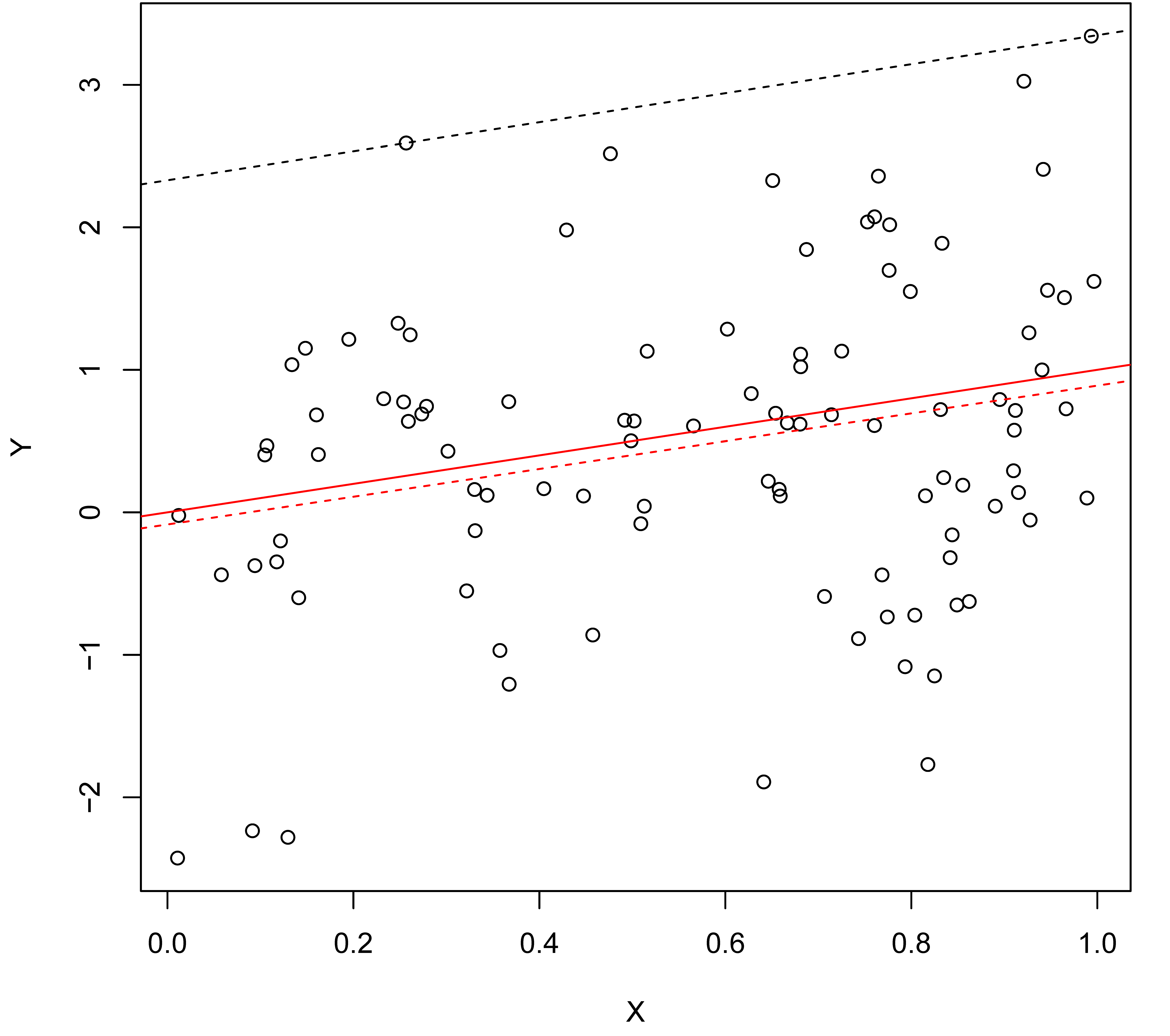
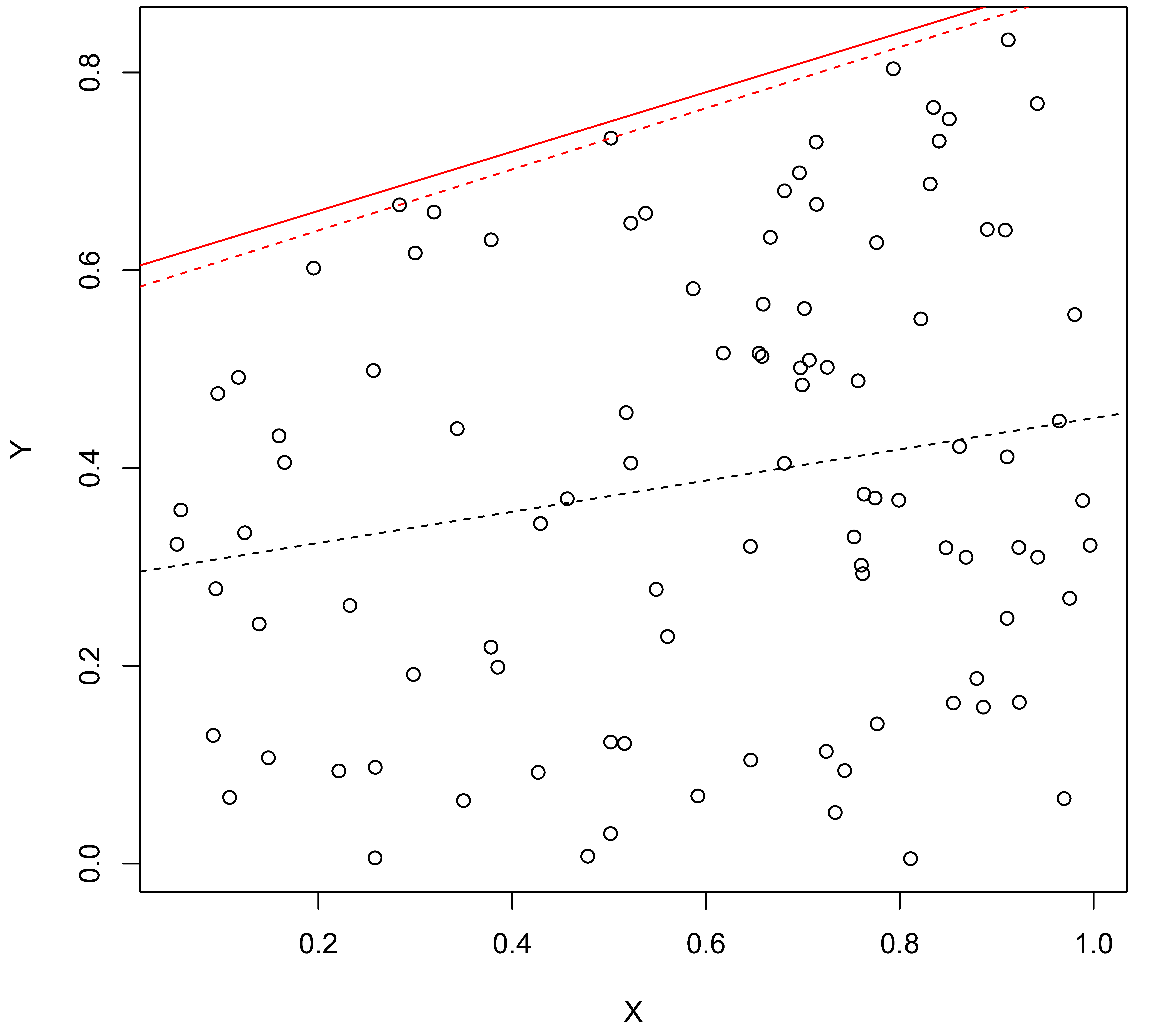
Correlation by probabilistic sufficiency (Left) and by necessity (Right). Random samples (n = 100) from a population with probabilistic sufficiency (solid line, Left) and necessity (solid line, Right). The dashed lines are estimated lines by OLS regression (center lines) and by NCA (ceiling lines).

Figure G.1: Correlation by probabilistic sufficiency (Left) and by necessity (Right). Random samples (n = 100) from a population with probabilistic sufficiency (solid line, Left) and necessity (solid line, Right). The dashed lines are estimated lines by OLS regression (center lines) and by NCA (ceiling lines).

Figure G.1 Right shows a similar $XY$-plot in which the solid line now represents a true linear necessity relationship in the population. The population data were generated with bounded variables $X$ and $Y$ with values between 0 and 1 and a uniform distribution below the ceiling (see Section 5.4). A sample of 100 cases was randomly drawn from this population and the relationship was estimated with the NCA’s C-LP ceiling line (solid line at the top). This shows that the estimated and the true necessity relationship are very close. The sample correlation coefficient is 0.19. The estimated OLS regression line in the center of the data (dotted line) illustrates that regression analysis does not capture the underlying necessity relationship in the population. The correlation is only an artifact of the necessity relationship due to the selected distribution of data below the ceiling.

The examples show that both types of relationships can produce a correlation coefficient. Since in these examples the data generation process is known, namely induced probabilistic sufficiency and necessity, respectively, it is easy to conclude in which situation the regression line and in which situation the ceiling line best represents the causal relationship in the population whereas the observed correlation is not informative for this. Unfortunately, in empirical studies the true causal relationship in the population is unknown, and an observed correlation does not tell what the underlying relationship was: probabilistic sufficiency, necessity or something else. Usually the analyst decides (e.g., based on theory) whether the underlying causality is probabilistic sufficiency, necessity (or both), and selects the appropriate estimation technique(s) accordingly. It is incorrect to assume a probabilistic relationship and apply NCA, just as it is inappropriate to assume a necessity relationship and apply regression analysis. Both represent a mismatch between theory and method, leading to a theory-method misfit (see Section 11.2). The often implicit assumption that the correlation coefficient indicates the presence of a probabilistic sufficiency relationship is incorrect if the underlying causality is necessity, but there is no way to evaluate this. The use of an (implicit) automatism to select probabilistic sufficiency as the underlying causality may have two reasons. First, this causal perspective is currently the main paradigm of causality. Second, the correlation coefficient $r$ and the regression coefficient $b$ are closely related and can be expressed by a simple mathematical equation (see Equation (G.1)).

A similar simple mathematical equation for the relationship between the regression coefficient and the correlation coefficient as in Equation (G.1) is not available for the relationship between necessity effect size and correlation coefficient. However, with certain assumptions, such a relationship can be derived. The general equation for the correlation coefficient can be written as:

\[\begin{aligned} \rho_{XY} & = \frac{{{E}}(XY) - {{E}}(X) {{E}}(Y)}{\sqrt{{{E}}(X^2) - {{E}}(X)^2} \sqrt{{{E}}(Y^2) - {{E}}(Y)^2}} \\\end{aligned}\]

where $\rho_{XY}$ is the Pearson correlation coefficient, and $E$ is the expected value.

For a linear ceiling line $f(x) = a + bx$ and a uniform distribution under the ceiling and within the bounding box (unit box), the correlation coefficient can be derived analytically, as shown below.¹²⁵

Situation

Consider a linear case with a tight bounding box (unit box): $0 < a <1 < a+b$.

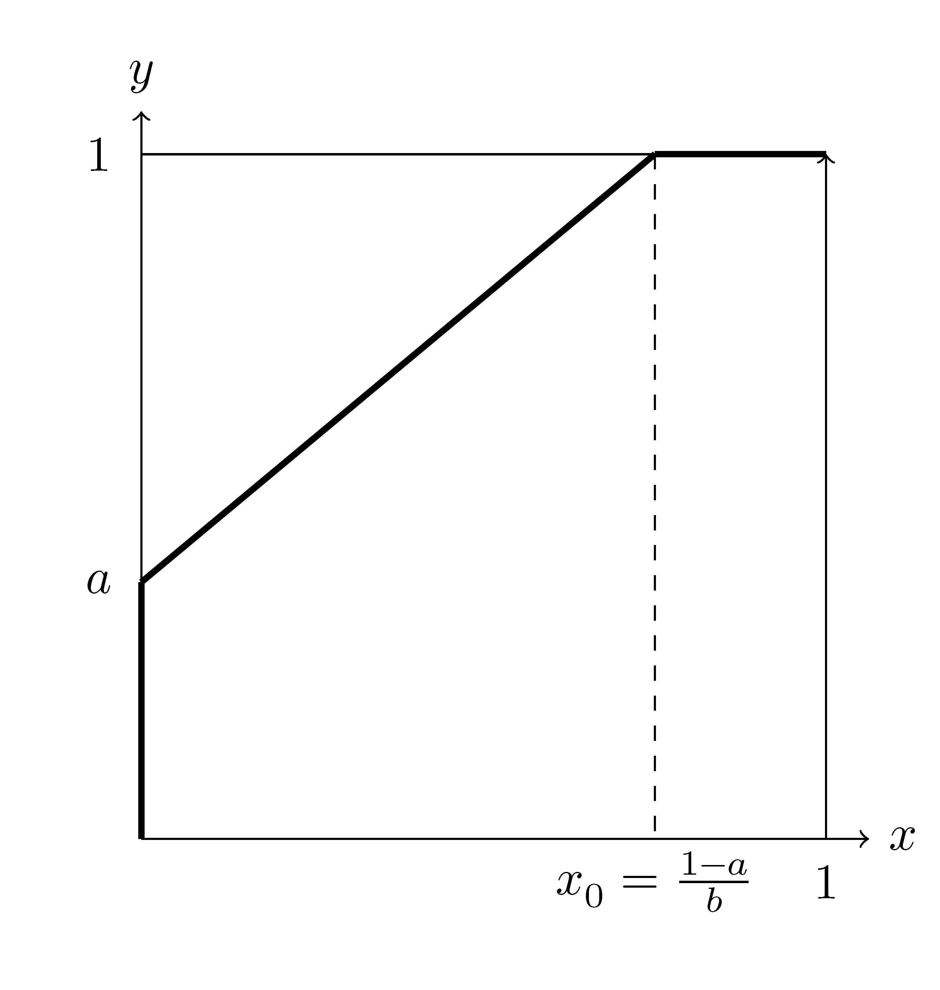
Figure G.2: Parameters: $0 < a < 1 < a+b$.

Define $L(x) = \min\{1,a+bx\}$. \[\begin{align} F_{a,b} & \equiv \int_0^1 L(x) \,dx = \text{surface area below thick line} \\ & = 1 - \text{surface area above thick line} \\ & = 1 - \tfrac{1}{2} (1-a) x_0 = 1 - \frac{(1-a)^2}{2b} \end{align}\] Uniform distribution $(X,Y)$ below the ceiling line: \[\begin{align} X & \propto \frac{1}{F_{a,b}} L(x) \,dx \\ Y|X & \propto \frac{I_{[0,L(x)]}(y)}{L(x)} \,dy \end{align}\] where $X$ is a random variable, $Y|X$ is a random variable $Y$ conditioned on $X$ and $\propto$ means `distributed with a density function given as’. Further, $I_{[0,L(x)]}$ is the indicator function for the interval $[0,L(x)]$. Note that \[ (X,Y) \propto \frac{1}{F_{a,b}} I_{[0,L(x)]}(y) \,dx \, \,dy = \frac{1}{F_{a,b}} I_{ y \leq a + bx}(x,y) \,dx \, \,dy \] is indeed the (normalized) uniform distribution below the line .

The text below uses four values, $a$, $b$, $x_0$, and $F_{a,b}$ to formulate expressions. Two are all that are needed. Indeed, for example, \[\begin{align*} \frac{1-F_{a,b}}{x_0} & = \frac{\frac{(1-a)^2}{2b}}{(1-a)/b} = \tfrac{1}{2} (1-a) \end{align*}\] and so \[ a = 1- 2 \frac{1-F_{a,b}}{x_0} \quad \text{or} \quad x_0 = 2 \frac{1-F_{a,b}}{1-a} \quad \text{or} \quad F_{a,b} = 1 - x_0 (1-a)/2 . \] Likewise \[ b = (1-a)/x_0 = \left( \frac{1- 2 \frac{1-F_{a,b}}{x_0}}{x_0} \right) .\]

Symmetry transformation

Consider the `double flip + transposition’ transformation: \[ (x,y) \mapsto (\alpha,\beta) \equiv (1-y,1-x) . \] In $\alpha\beta$ coordinates Figure G.2 presents itself as Figure G.3.

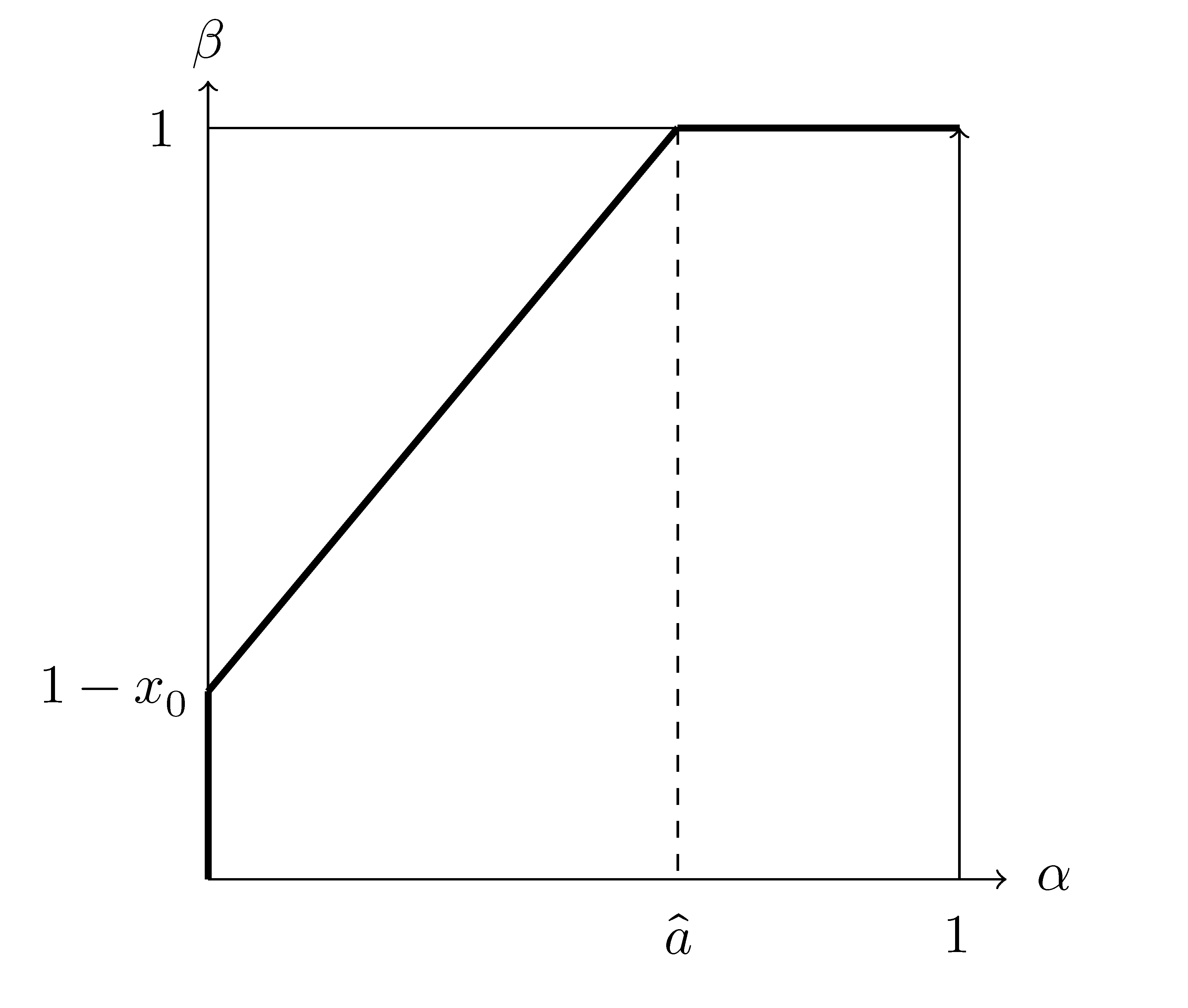
$Parameters: $\hat{a}=1-a$ with $0 < \hat{a} < 1$ and $0 < x_0 < 1$.$

Figure G.3: Parameters: $\hat{a}=1-a$ with $0 < \hat{a} < 1$ and $0 < x_0 < 1$.

The ceiling function in $\alpha \beta$ coordinates is $\hat{L}(\alpha) = \min(1, (1-x_0) + (1/b) \beta$. Now \[ E{Y} = E(1-\alpha) = 1 - E(\alpha) \] where, by symmetry, \[ E(\alpha) = E(X) \quad [\text{where $x_0 \leftrightarrow \hat{a}$}] . \] Note that under the symmetry $x_0 \leftrightarrow \hat{a}$ the value of $F_{a,b} = 1 - \tfrac{1}{2} x_0 \hat{a}$ is evidently invariant.

Correlation

\[ \rho_{XY} = \frac{E(XY) - E(X) E(Y)}{\sigma_X \sigma_Y} . \] Five integrals:

Expectation of $X$.

\[\begin{align*} E(X) &= \frac{1}{F_{a,b}} \int_0^1 x L(x)\,dx \\ &= \frac{1}{F_{a,b}} \int_0^1 x \min\{1,a+bx\}\,dx\\ &= \frac{1}{F_{a,b}} \left( \int_0^{(1-a)/b} (ax + bx^2)\,dx + \int_{(1-a)/b}^1 x\,dx \right) \\ &= \frac{1}{F_{a,b}} \left( \left.(\tfrac{1}{2}ax^2 + \tfrac{1}{3}bx^3)\right|_{0}^{(1-a)/b} + \left.\tfrac{1}{2}x^2\right|_{(1-a)/b}^{1} \right) \\ &= \frac{1}{F_{a,b}} \left( \tfrac{1}{2}a \left(\frac{1-a}{b}\right)^2 + \tfrac{1}{3}b\left(\frac{1-a}{b}\right)^3 + \tfrac{1}{2} - \tfrac{1}{2} \left(\frac{1-a}{b}\right)^2 \right)\\ &= \frac{1}{2F_{a,b}} \left( 1 + (a + \tfrac{2}{3}(1-a) + 1)\left(\frac{1-a}{b}\right)^2 \right) \\ &= \frac{1}{2F_{a,b}} \left( 1 - \tfrac{1}{3}(1-a)\left(\frac{1-a}{b}\right)^2 \right) \\ &= \frac{1}{2F_{a,b}} \left( \tfrac{2}{3}\frac{(1-a)}{b} - \tfrac{2}{3}\frac{(1-a)}{b}\frac{(1-a)^2}{2b} + 1 - \tfrac{2}{3}\frac{(1-a)}{b} \right) \\ &= \frac{1}{2F_{a,b}} \left( \tfrac{2}{3}\frac{(1-a)}{b}F_{a,b} + 1 - \tfrac{2}{3}\frac{(1-a)}{b} \right) \\ &= \tfrac{1}{2} \left( \tfrac{2}{3}\frac{(1-a)}{b} + \left(1 - \tfrac{2}{3}\frac{(1-a)}{b}\right)\frac{1}{F_{a,b}} \right) \\ &= \tfrac{1}{2} \left( \tfrac{2}{3}x_0 + \left(1 - \tfrac{2}{3}x_0\right)\frac{1}{F_{a,b}} \right)\\ &= \frac{1}{2F_{a,b}} \left( 1 - \tfrac{2}{3}x_0 + \tfrac{2}{3}x_0 F_{a,b} \right). \end{align*}\]

Note. As $\frac{1}{F_{a,b}} \geq 1$ we have

\[ E(X) = \tfrac{1}{2} \left( \tfrac{2}{3} x_0 + \left( 1 - \tfrac{2}{3} x_0 \right) \frac{1}{F_{a,b}} \right) \geq \tfrac{1}{2} \left( \tfrac{2}{3} x_0 + 1 - \tfrac{2}{3} x_0 \right) = \tfrac{1}{2} \]

as is evident from Figure G.2. Reworking $E(X)$ (into $\hat{a}$ and $x_0$) we obtain

\[\begin{align*} E(X) &= \frac{1}{2F_{a,b}} \left( 1 - \tfrac{2}{3} x_0 + \tfrac{2}{3} x_0 F_{a,b} \right) \\ &= \frac{1}{2F_{a,b}} \left( 1 - \tfrac{2}{3} x_0 + \tfrac{2}{3} x_0 (1-\tfrac{1}{2} \hat{a} x_0) \right) \\ &= \frac{1}{2F_{a,b}} \left( 1 - \tfrac{1}{3} \hat{a}\,x_0^2 \right). \end{align*}\]

Expectation of $Y$. Note that $E(Y) = E(E(Y \mid X))$.

Step 1.

\[ E(Y \mid X=x) = \int_0^{L(x)} y \frac{I_{[0,L(x)]}(y)}{L(x)}\,dy = \left.\tfrac{1}{2}\frac{y^2}{L(x)}\right|_{0}^{L(x)} = \tfrac{1}{2}L(x). \]

Step 2.

\[\begin{align*} E(Y) &= \int_0^{1} \tfrac{1}{2} L(x)\frac{L(x)}{F_{a,b}}\,dx \\ &= \frac{1}{2F_{a,b}} \left( \int_0^{(1-a)/b} (a+bx)^2\,dx + \int_{(1-a)/b}^1\,dx \right) \\ &= \frac{1}{2F_{a,b}} \left( \int_0^{(1-a)/b} (a^2 + 2abx + b^2x^2)\,dx + \int_{(1-a)/b}^1\,dx \right) \\ &= \frac{1}{2F_{a,b}} \left( \left.(a^2x + abx^2 + \tfrac{1}{3}b^2x^3)\right|_{0}^{(1-a)/b} + \left.x\right|_{(1-a)/b}^{1} \right) \\ &= \frac{1}{2F_{a,b}} \left( a^2 \frac{1-a}{b} + ab\left(\frac{1-a}{b}\right)^2 + \tfrac{1}{3} b^2\left(\frac{1-a}{b}\right)^3 + 1 - \frac{1-a}{b} \right) \\ &= \frac{1}{2F_{a,b}} \left( a^2 x_0 + 2a \frac{(1-a)^2}{2b} + \tfrac{2}{3}(1-a)\frac{(1-a)^2}{2b} + 1 - x_0 \right) \\ &= \frac{1}{2F_{a,b}} \left( a^2 x_0 + (2a + \tfrac{2}{3}(1-a))(1 - F_{a,b}) + 1 - x_0 \right) \\ &= \frac{1}{2F_{a,b}} \left( 1 - x_0 + a^2 x_0 + \tfrac{2}{3}(2a + 1)(1 - F_{a,b}) \right) \\ &= \frac{1}{2F_{a,b}} \left( 1 + (a-1)(a+1)x_0 + \tfrac{2}{3}(2a + 1)(1 - F_{a,b}) \right) \\ &= \frac{1}{2F_{a,b}} \left( 1 - 2(a+1)(1-F_{a,b}) + \tfrac{2}{3}(2a + 1)(1 - F_{a,b}) \right) \\ &= \frac{1}{2F_{a,b}} \left( 1 - \tfrac{2}{3}(a+2)(1-F_{a,b}) \right) \\ &= \frac{1}{2F_{a,b}} \left( 1 - \tfrac{2}{3}(a+2) + \tfrac{2}{3}(a+2)F_{a,b} \right). \end{align*}\]

Set $\theta(a) = \tfrac{1}{3}(a+2) \leq \tfrac{1}{3}(1+2) = 1$. Also, evidently $\theta(a) \geq \tfrac{2}{3}$. Now

\[\begin{align*} E(Y) &= \frac{1}{2F_{a,b}} ( 1 - 2\theta(a) + 2\theta(a) F_{a,b} ) \\ &= \frac{1}{2F_{a,b}} \left( 1 - 2\theta(a)(1 - F_{a,b}) \right) \\ &\leq \frac{1}{2F_{a,b}} \left( 1 - \tfrac{4}{3}(1 - F_{a,b}) \right) \\ &= \frac{1}{2F_{a,b}} \left( - \tfrac{1}{3} + \tfrac{4}{3} F_{a,b} \right) \\ &= \frac{1}{2} \left( - \tfrac{1}{3}\frac{1}{F_{a,b}} + \tfrac{1}{3} + 1 \right) \leq \frac{1}{2}. \end{align*}\]

Note that the final inequality is strict for $F_{a,b} < 1$. The inequality $E(Y) \leq \tfrac{1}{2}$ is evident from Figure G.2.

Alternative calculation.

Note that

\[\begin{align*} a^2 (1-a) + a(1-a)^2 + \tfrac{1}{3} (1-a)^3 &= a^2-a^3 + a(1-2a+a^2) + \tfrac{1}{3} (1-a)(1-2a+a^2) \\ &= a - a^2 + \tfrac{1}{3} (1-2a+a^2-a+2a^2-a^3) \\ &= a - a^2 + \tfrac{1}{3}(1-a^3) - a + a^2 = \tfrac{1}{3}(1-a^3). \end{align*}\]

Also note

\[ (1-a^3) = (1-a) (3a + (1-a)^2) = (1-a) (3a + 1-2a + a^2) = (1-a) (1 + a + a^2). \]

Reworking $E(Y)$ (into $\hat{a}$ and $x_0$) using the symmetry

\[\begin{align*} E(Y) &= \frac{1}{2F_{a,b}} \left( 1 - \tfrac{2}{3}(a+2) + \tfrac{2}{3}(a+2) F_{a,b} \right) \\ &= \frac{1}{2F_{a,b}} \left( 1 - \tfrac{2}{3}(1-\hat{a}+2) + \tfrac{2}{3}(1-\hat{a}+2)(1-\tfrac{1}{2} x_0 \hat{a}) \right) \\ &= \frac{1}{2F_{a,b}} \left( 1 - \tfrac{1}{3}(3-\hat{a}) x_0 \hat{a} \right) \\ &= 1 - \frac{1}{2F_{a,b}} \left( -1 + 2 F_{a,b} + \tfrac{1}{3}(3-\hat{a}) x_0 \hat{a} \right) \\ &= 1 - \frac{1}{2F_{a,b}} \left( -1 + 2 - x_0 \hat{a} + \tfrac{1}{3}(3-\hat{a}) x_0 \hat{a} \right) \\ &= 1 - \frac{1}{2F_{a,b}} \left( 1 - \tfrac{1}{3} x_0 \hat{a}^2 \right) = 1 - E(X)\,[\text{where $x_0 \leftrightarrow \hat{a}$}]. \end{align*}\]

Second moment of $X$.

\[\begin{align*} E(X^2) &= \frac{1}{F_{a,b}} \int_0^1 x^2 L(x)\,dx \\ &= \frac{1}{F_{a,b}} \int_0^1 x^2 \min\{1,a+bx\}\,dx\\ &= \frac{1}{F_{a,b}} \left( \int_0^{(1-a)/b} (ax^2 + bx^3)\,dx + \int_{(1-a)/b}^1 x^2\,dx \right) \\ &= \frac{1}{F_{a,b}} \left( \left.(\tfrac{1}{3}ax^3 + \tfrac{1}{4}bx^4)\right|_{0}^{(1-a)/b} + \left.\tfrac{1}{3}x^3\right|_{(1-a)/b}^{1} \right) \\ &= \frac{1}{F_{a,b}} \left( \tfrac{1}{3}a \left(\frac{1-a}{b}\right)^3 + \tfrac{1}{4}b\left(\frac{1-a}{b}\right)^4 + \tfrac{1}{3} - \tfrac{1}{3} \left(\frac{1-a}{b}\right)^3 \right)\\ &= \frac{1}{F_{a,b}} \left( \tfrac{1}{3} - \tfrac{8}{3}(1-a)\left(\frac{1-a}{2b}\right)^3 + 2(1-a)\left(\frac{1-a}{2b}\right)^3 \right)\\ &= \frac{1}{F_{a,b}} \left( \tfrac{1}{3} - \tfrac{8}{3}\left(\frac{(1-a)}{2b}\right)^2 \left(\frac{(1-a)^2}{2b}\right) + 2\left(\frac{(1-a)}{2b}\right)^2 \left(\frac{(1-a)^2}{2b}\right) \right)\\ &= \frac{1}{F_{a,b}} \left( \tfrac{1}{3} - \tfrac{2}{3} x_0^2 (1-F_{a,b}) + \tfrac{1}{2} x_0^2 (1-F_{a,b}) \right) \\ &= \frac{1}{F_{a,b}} \left( \tfrac{1}{3} - \tfrac{1}{6} x_0^2 (1-F_{a,b}) \right) \\ &= \frac{1}{3F_{a,b}} \left( (1 - \tfrac{1}{2} x_0^2) + \tfrac{1}{2} x_0^2 F_{a,b} \right). \end{align*}\]

Second moment of $Y$. Note $E(Y^2) = E(E(Y^2 \mid X))$.

Step 1.

\[ E(Y^2 \mid X=x) = \int_0^{L(x)} y^2 \frac{I_{[0,L(x)]}(y)}{L(x)}\,dy = \left.\tfrac{1}{3}\frac{y^3}{L(x)}\right|_{0}^{L(x)} = \tfrac{1}{3}(L(x))^2. \]

Step 2.

Note that $1-a^4 = (1-a)(1+a+a^2+a^3) = (1-a^3) + (1-a)a^3$. Also, $1-a^4 = (1-a^2)(1+a^2) = (1-a)(1+a)(1+a^2)$. We continue:

\[\begin{align*} E(Y^2) &= \frac{1}{3F_{a,b}} \left( \frac{1}{4b} (1-a)(1+a)(1+a^2) + 1 - \frac{1-a}{b} \right). \end{align*}\]

Alternative:

\[\begin{align*} E(Y^2) &= \int_0^{1} \tfrac{1}{3}(L(x))^2 \frac{L(x)}{F_{a,b}}\,dx \\ &= \frac{1}{3F_{a,b}} \left( \int_0^{(1-a)/b} (a+bx)^3\,dx + \int_{(1-a)/b}^1\,dx \right) \\ &= \frac{1}{3F_{a,b}} \left( \int_0^{(1-a)/b} (a^3 + 3a^2bx + 3ab^2x^2 + b^3x^3)\,dx + \left.x\right|_{(1-a)/b}^{1} \right) \\ &= \frac{1}{3F_{a,b}} \left( \left.a^3x + \tfrac{1}{2} 3a^2bx^2 + ab^2x^3 + \tfrac{1}{4}b^3x^4\right|_{0}^{(1-a)/b} + 1 - \frac{1-a}{b} \right) \\ &= \frac{1}{3F_{a,b}} \left( a^3\frac{1-a}{b} + \tfrac{3}{2} a^2b\left(\frac{1-a}{b}\right)^2 + ab^2\left(\frac{1-a}{b}\right)^3 + \tfrac{1}{4}b^3\left(\frac{1-a}{b}\right)^4 + 1 - \frac{1-a}{b} \right) \\ &= \frac{1}{3F_{a,b}} \left( a^3 x_0 + 3 a^2 (1-F_{a,b}) + 2a(1-a) (1-F_{a,b}) + \tfrac{1}{2} (1-a)^2 (1-F_{a,b}) + 1 - x_0 \right) \\ &= \frac{1}{3F_{a,b}} \left(1 - (1 - a^3) x_0 + \left(3 a^2 + 2a(1-a) + \tfrac{1}{2} (1-a)^2 \right) (1-F_{a,b}) \right) \\ &= \frac{1}{3F_{a,b}} \left(1 - (1 - a^3) x_0 + \left(3a^2 + 2a - 2a^2 + \tfrac{1}{2} - a + \tfrac{1}{2} a^2 \right) (1-F_{a,b}) \right). \end{align*}\]

Continuing:

\[\begin{align*} E(Y^2) &= \frac{1}{3F_{a,b}} \left(1 - (1 - a^3) x_0 + \left(\tfrac{1}{2} + a + \tfrac{3}{2} a^2 \right) (1-F_{a,b}) \right) \\ &= \frac{1}{3F_{a,b}} \left(1 - (1 - a)(1+a+a^2) \frac{1-a}{b} + \left(\tfrac{1}{2} + a + \tfrac{3}{2} a^2 \right) (1-F_{a,b}) \right) \\ &= \frac{1}{3F_{a,b}} \left(1 - 2(1+a+a^2) (1-F_{a,b}) + \left(\tfrac{1}{2} + a + \tfrac{3}{2} a^2 \right) (1-F_{a,b}) \right) \\ &= \frac{1}{3F_{a,b}} \left(1 - \tfrac{1}{2} (3 + 2a + a^2) (1-F_{a,b}) \right) \\ &= \frac{1}{3F_{a,b}} \left(- \tfrac{1}{2} - a - \tfrac{1}{2}a^2 + \tfrac{1}{2} (3 + 2a + a^2) F_{a,b} \right) \\ &= \frac{1}{3F_{a,b}} \left( -\tfrac{1}{2} (1+a)^2 + (1 + \tfrac{1}{2} (1+a)^2) F_{a,b} \right) \\ &= \frac{1}{3F_{a,b}} \left( -\tfrac{1}{2} (2-\hat{a})^2 + (1 + \tfrac{1}{2} (2-\hat{a})^2) F_{a,b} \right). \end{align*}\]

Verification via symmetry:

\[\begin{align*} E(Y^2) &= E((1-\alpha)^2) = 1 - 2E(\alpha) + E(\alpha^2) \\ &= 1 - 2E(X)[\text{where $x_0 \leftrightarrow \hat{a}$}] + E(X^2)[\text{where $x_0 \leftrightarrow \hat{a}$}] \\ &= 1 - \frac{1}{F_{a,b}} (1 - \tfrac{1}{3} x_0 \hat{a}^2) + \frac{1}{3F_{a,b}} (1 - \tfrac{1}{2}\hat{a}^2 + \frac{1}{2}\hat{a}^2 F_{a,b}) \\ &= \frac{1}{3F_{a,b}} \left( 3F - 3(1 - \tfrac{1}{3} x_0 \hat{a}^2) + 1 - \tfrac{1}{2}\hat{a}^2 + \frac{1}{2}\hat{a}^2 F_{a,b} \right) \\ &= \frac{1}{3F_{a,b}} \left( -2 - \tfrac{1}{2}\hat{a}^2 + x_0 \hat{a}^2 + (3 + \tfrac{1}{2}\hat{a}^2) F_{a,b} \right) \\ &= \frac{1}{3F_{a,b}} \left( -2 - \tfrac{1}{2}\hat{a}^2 + 2\hat{a} (1-F_{a,b}) + (3 + \tfrac{1}{2}\hat{a}^2) F_{a,b} \right) \\ &= \frac{1}{3F_{a,b}} \left( -2 + 2\hat{a} - \tfrac{1}{2}\hat{a}^2 + (1 + 2 - 2\hat{a} + \tfrac{1}{2}\hat{a}^2) F_{a,b} \right) \\ &= \frac{1}{3F_{a,b}} \left( - \tfrac{1}{2} (2-\hat{a})^2 + (1 + \tfrac{1}{2} (2-\hat{a})^2) F_{a,b} \right). \end{align*}\]

Inner product $E(XY)$. We have $E(XY) = E(E(XY \mid X=x))$.

Step 1.

\[\begin{align*} E(XY \mid X=x) &= x \int_0^{L(x)} y \frac{I_{[0,L(x)]}}{L(x)}(y)\,dy \\ &= \frac{x}{L(x)} \left.\tfrac{1}{2} y^2\right|_{0}^{L(x)} \\ &= \tfrac{1}{2} x L(x). \end{align*}\]

Step 2.

\[\begin{align*} E(XY) &= \frac{1}{F_{a,b}} \int_0^1 \tfrac{1}{2} x (L(x))^2\,dx \\ &= \frac{1}{2F_{a,b}} \left( \int_0^{(1-a)/b} x(a+bx)^2\,dx + \int_{(1-a)/b}^1 x\,dx \right) \\ &= \frac{1}{2F_{a,b}} \left( \int_0^{(1-a)/b} (a^2x + 2abx^2 + b^2x^3)\,dx + \tfrac{1}{2} \left.x^2\right|_{(1-a)/b}^{1} \right) \\ &= \frac{1}{2F_{a,b}} \left( \left.(\tfrac{1}{2}a^2x^2 + \tfrac{2}{3}abx^3 + \tfrac{1}{4}b^2x^4)\right|_{0}^{(1-a)/b} + \tfrac{1}{2} \left( 1 - \left(\frac{1-a}{b}\right)^2 \right) \right) \\ &= \frac{1}{4F_{a,b}} \left( 1 - \left(\frac{1-a}{b}\right)^2 + a^2\left(\frac{1-a}{b}\right)^2 + \tfrac{4}{3}ab\left(\frac{1-a}{b}\right)^3 + \tfrac{1}{2}b^2\left(\frac{1-a}{b}\right)^4 \right)\\ &= \frac{1}{4F_{a,b}} \left( 1 - (1+a) \frac{(1-a)^3}{b^2} + \tfrac{4}{3}a(1-a)/b \frac{(1-a)^2}{b} + \tfrac{1}{2}(1-a)^2/b \frac{(1-a)^2}{b} \right)\\ &= \frac{1}{4F_{a,b}} \left( 1 + \left(-2(1+a)x_0 + \tfrac{8}{3}ax_0 + (1-a)x_0 \right) (1-F_{a,b}) \right)\\ &= \frac{1}{4F_{a,b}} \left( 1 + \left( -x_0 - \tfrac{1}{3}ax_0 \right) (1-F_{a,b}) \right) \\ &= \frac{1}{4F_{a,b}} \left( 1 - x_0 - \tfrac{1}{3}ax_0 + (x_0 + \tfrac{1}{3}ax_0) F_{a,b} \right). \end{align*}\]

Note that

\[ x_0 + \tfrac{1}{3}ax_0 = x_0 + \tfrac{1}{3}(1-\hat{a})x_0 = \tfrac{2}{3}(2x_0 - 1 + F_{a,b}). \]

and so

\[\begin{align*} E(XY) &= \frac{1}{4F_{a,b}} \left( 1 + \tfrac{2}{3} (1 - 2x_0 - F_{a,b}) - \tfrac{2}{3} (1 - 2x_0 - F_{a,b}) F_{a,b} \right) \\ &= \frac{1}{4F_{a,b}} \left( 1 - \tfrac{2}{3} (2x_0 + F_{a,b}) + \tfrac{2}{3} (2x_0 + F_{a,b}) F_{a,b} \right) \\ &= \frac{1}{4F_{a,b}} \left( 1 - \tfrac{2}{3} (2x_0 + F_{a,b}) (1 - F_{a,b}) \right). \end{align*}\]

Therefore the correlation is:

\[ \begin{aligned} \rho_{XY} & = \frac{{{E}}(XY) - {{E}}(X) {{E}}(Y)} {\sqrt{{{E}}(X^2) - {{E}}(X)^2} \sqrt{{{E} }(Y^2) - {{E}}(Y)^2}} = \\\end{aligned} \]

\[\begin{aligned} \frac{ \frac{1}{4F_{a,b}} \left( 1 - x_0 - \tfrac{1}{3}ax_0 + (x_0 + \tfrac{1}{3}ax_0)F_{a,b} \right) - \frac{1}{2F_{a,b}} \left( 1 - \tfrac{2}{3}x_0 + \tfrac{2}{3}x_0F_{a,b} \right) \frac{1}{2F_{a,b}} \left( 1 - \tfrac{2}{3}(a+2) + \tfrac{2}{3}(a+2)F_{a,b} \right) }{ \sqrt{ \frac{1}{3F_{a,b}} \left( 1 - \tfrac{1}{2}x_0^2 + \tfrac{1}{2}x_0^2F_{a,b} \right) - \left( \frac{1}{2F_{a,b}} \left( 1 - \tfrac{2}{3}x_0 + \tfrac{2}{3}x_0F_{a,b} \right) \right)^2 } \sqrt{ \frac{1}{3F_{a,b}} \left( -\tfrac{1}{2}(1+a)^2 + \left( 1 + \tfrac{1}{2}(1+a)^2 \right)F_{a,b} \right) - \left( \frac{1}{2F_{a,b}} \left( 1 - \tfrac{2}{3}(a+2) + \tfrac{2}{3}(a+2)F_{a,b} \right) \right)^2 } }. \end{aligned}\]

The derivation was done by Roelof Kuik.↩︎